In this blog post, we explore the coefficient of variation in R, a measure of relative variability. Ths coefficient expresses the standard deviation as a percentage of the mean, telling us about our data’s variability. We will cover the formula and interpretation.
Throughout the post, we will learn how to calculate and visualize the coefficient of variation using base R, the dplyr, and the ggplot2 packages. First, however, we will look at an example from psychological science to illustrate its application. By the end, you will hopefully grasp how to calculate the coefficient of variation in R.
Now, let us outline the post to structure our discussion and provide a clear path to learning about the coefficient of variation in R. You might also find the calculator useful:
Table of Contents
- Outline
- Coefficient of Variation
- Example from Psychology
- Prerequisites
- Synthetic Data
- How to Find the Coefficient of Variation with Base R
- How to Calculate the Coefficient of Variation in R with dplyr
- Coefficients of Variation for all Numeric Variables
- Calculate Coefficient of Variation by Group in R
- Calculate Coefficient of Variation by Group for all Numeric Variables in R
- Plot the Coefficient of Variation in R
- Conclusion
- R Tutorials
Outline
The first section will cover the concept of the coefficient of variation and its interpretation. We will explain how it expresses the standard deviation as a percentage of the mean. Next, we will discuss an example from Psychological research to illustrate the practical application of the coefficient of variation.
In the subsequent section, we will outline the prerequisites for this post. It is important to have basic knowledge of R programming and familiarity with base R functions. We will generate synthetic data containing the reaction times of two groups to facilitate practice (or following the exact examples of the post). We will then learn the different methods of calculating the coefficient of variation. First, we will explore how to find the coefficient of variation using base R functions, such as mean() and sd().
Next, we will demonstrate how to calculate the coefficient of variation in R using the dplyr package. Leveraging dplyr’s group_by(), summarise(), and across() functions, we will efficiently compute the coefficient of variation for multiple variables simultaneously. Furthermore, we will cover how to calculate the coefficient of variation by group in R. We will also expand our analysis to calculate the coefficient of variation by group for all numeric variables in R. Finally, we will explore the visualization aspect by plotting the coefficient of variation in R.
Coefficient of Variation
The coefficient of variation is a statistical measure that quantifies a dataset’s relative variability. It expresses the standard deviation as a percentage of the mean, providing insights into the dispersion of values concerning their average. The formula is simple: divide the standard deviation by the mean and multiply by 100. This normalization allows for a standardized comparison of variability across different datasets, regardless of their scales or units.
CV = (σ / μ) * 100
where:
- σ (standard deviation): A measure of the dataset’s dispersion or spread of values.
- μ (mean): The average value of the dataset.
The coefficient of variation is handy when comparing datasets with different means, as it considers the proportion of variation relative to the average value. A higher coefficient indicates greater relative variability, suggesting a wider spread of data points around the mean. Conversely, a lower coefficient of variation implies greater consistency and less dispersion among the values.
Interpretation
Interpreting the coefficient of variation depends on the context of the data. In fields such as finance and economics, a higher coefficient of variation may indicate higher risk or volatility, whereas a lower coefficient of variation suggests stability. In scientific research, the coefficient of variation helps assess the consistency and reliability of measurements or experimental outcomes.
By calculating the coefficient of variation, we gain valuable insights into the relative variability of our data, which can inform decision-making and guide further analysis. It enables us to identify datasets with high dispersion or wide fluctuations and focus on understanding the factors contributing to the variability.
In summary, the coefficient of variation is a powerful tool for measuring and comparing the relative variability of datasets. Its formula, which normalizes the standard deviation by the mean, allows for standardized comparisons across different datasets. Understanding the coefficient of variation helps us grasp the spread and stability of our data, providing insights that aid decision-making and enhance our understanding of data patterns.
Example from Psychology
In Psychological Science, the coefficient of variation is helpful in various applications. For instance, let us consider a research study examining reaction times (RT) in a cognitive task. RT is a crucial measure that reflects cognitive processing speed and can provide valuable insights into cognitive functioning.
Suppose we compare the reaction times of Group A and Group B. In this example, we want to determine which group exhibits more significant variability in their RT. By calculating the coefficient for each group, we can assess the relative variability of their reaction times compared to their respective means.
If Group A has a higher coefficient of variation than Group B, it suggests that the RTs within Group A are more widely dispersed relative to their mean. This may indicate more significant inconsistency or fluctuations in cognitive processing speed within Group A. On the other hand, if Group B has a lower coefficient, it suggests more consistency in their RTs and less variability around the mean.
Employing the coefficient of variation here can help us gain insights into the relative variability of RTs between groups. This information can contribute to a better understanding of cognitive processes, such as attention, memory, or decision-making, and potentially shed light on underlying individual differences or group characteristics.
In conclusion, the coefficient of variation can serve as a tool in Psychological Science to quantify and compare the relative variability of data. It enables us to explore patterns, identify differences, and interpret the spread of values concerning the mean, providing valuable insights into the phenomena under investigation.
Prerequisites
To follow this tutorial on the coefficient of variation in R, you will need a basic understanding of R programming. Familiarity with concepts like data manipulation, data frames, and basic statistical calculations will also be helpful.
We will primarily use base R functions and packages like dplyr and DescTools. You can do so using the install if you have not installed these packages.packages() function in R. For example, to install dplyr, you can run install.packages(“dplyr”). Similarly, you can install ggplot2 by running install.packages(“ggplot2”).
The dplyr package provides a wide range of functions for data manipulation, such as renaming columns, selecting specific columns, sum across columns, and more. These functions can streamline your data preprocessing tasks. The ggplot2 package can be used to create scatter plots, violin plots, residual plots, and plot the prediction interval, amongst other things.
Lastly, updating R to the latest version is recommended to ensure you can access the most recent features and bug fixes. You can update R by, e.g., downloading and installing the latest stable version from the official R website.
Synthetic Data
Here is some synthetic data to practice calculating the coefficient of variation in R:
library(dplyr)

# Set the seed for reproducibility
set.seed(123)

# Define the reaction times for each group
group1_rt <- rnorm(100, mean = 500, sd = 100)
group2_rt <- rnorm(120, mean = 550, sd = 120)

# Create a grouping variable
group <- c(rep("Group 1", length(group1_rt)), rep("Group 2", length(group2_rt)))

# Create a condition variable using %in%
condition <- ifelse(group %in% "Group 1", "Condition A", "Condition B")

# Create an accuracy variable
accuracy <- c(sample(0:1, length(group1_rt),
                     replace = TRUE, prob = c(0.2, 0.8)),
              sample(0:1, length(group2_rt),
                     replace = TRUE, prob = c(0.4, 0.6)))

# Combine the reaction times, group, condition, and accuracy into a data frame
df <- data.frame(RT = c(group1_rt, group2_rt),
                 Group = group,
                 Condition = condition,
                 Accuracy = accuracy)

# Print the first few rows of the synthetic dataset
head(df)Code language: PHP (php)
In the code chunk above, we first load the dplyr package, which provides data manipulation and analysis functions in R. To ensure reproducibility, we set the seed value to 123 using set.seed(123). This allows us to generate the same random numbers each time we run the code.
We then define each group’s reaction times (RTs) using the rnorm() function. We generate 100 RTs for “Group 1” with a mean of 500 and a standard deviation of 100. Similarly, we generate 120 RTs for “Group 2” with a mean of 550 and a standard deviation of 120. Using the repeat (rep()) function, we create a grouping variable called “group”. Here we repeat the labels “Group 1” and “Group 2” corresponding to the number of RTs.
To create a condition variable named “condition”, we use the %in% in R. The %in% operator is used to assign “Condition A” if the group is “Group 1” and “Condition B” for all other groups.
We then combine the RTs, group, condition, and accuracy into a dataframe called “df” using the data.frame() function. The dataframe consists of four columns: “RT” representing the reaction times and “Group” indicating the group information. It also includes the “Condition” column denoting the condition information and the “Accuracy” column reflecting the accuracy values. We use the sample() function to randomly select values of 0 and 1 for the accuracy variable. The length of each group’s RTs is used as the size argument for sampling. We specify the replace = TRUE argument to allow sampling with replacement, and we set the probabilities for selecting 0 and 1 using the prob argument.
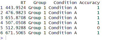
We utilize the head() function to examine the synthetic dataset’s structure and content. This function allows us to display the first few rows of the “df” dataframe. Here are the first six rows of the data:
How to Find the Coefficient of Variation with Base R
Here is how to calculate the coefficient of variation using base R:
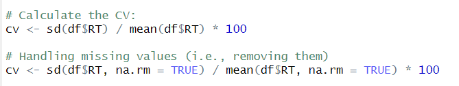
# Calculate the coefficient of variation using base R
cv <- sd(df$RT) / mean(df$RT) * 100Code language: R (r)
In the code chunk above, we calculate the coefficient of variation using base functions. Remember, the formula for the coefficient of variation is the standard deviation divided by the mean. This value is then multiplied by 100 to express it as a percentage.
By applying sd(df$RT) and mean(df$RT) to the reaction time data df$RT, we obtain the standard deviation and the mean, respectively. Dividing the standard deviation by the mean gives us the relative measure of variability. Multiplying it by 100 provides the coefficient of variation as a percentage. Importantly, if we have missing values in our data, we need to use the na.rm = TRUE argument.
cv <- sd(df$RT, na.rm = TRUE) / mean(df$RT, na.rm = TRUE) * 100Code language: R (r)This method calculates the coefficient of variation using the basic statistical functions available in R. It provides a straightforward approach to assessing the relative variability in the data.
How to Calculate the Coefficient of Variation in R with dplyr
Here is another way to find the coefficient of variation in R using the dplyr package:
library(dplyr)

# Calculate the coefficient of variation using dplyr
cv <- rt_data %>%
  summarise(cv = sd(RT) / mean(RT) * 100)Code language: R (r)
In the code chunk above, we utilize the dplyr package to calculate the coefficient of variation. We use the summarise() function to compute the coefficient of variation by dividing the standard deviation (sd(RT)) of the reaction time data (RT) by the mean (mean(RT)), and then multiply it by 100 to obtain the percentage.
By chaining the %>% operator, we pass the dataset rt_data to the summarise() function, which performs the required calculations. The resulting coefficient is stored in the cv variable.
In addition to calculating the coefficient of variation, the summarise() function in dplyr allows us to obtain various other summary statistics in R, such as mean, median, minimum, maximum, and more. This provides a convenient and efficient approach to performing R’s comprehensive data summarization and analysis tasks.
Coefficients of Variation for all Numeric Variables
If we want to summarize and calculate the coefficient of variation on all numeric vectors in a dataframe using dplyr, we can use the across() function. Here is an example:
library(dplyr)

# Calculate coefficient of variation for all numeric columns in the dataframe
summary_df <- rt_data %>%
  summarise(across(where(is.numeric), list(cv = ~sd(.)/mean(.) * 100)))Code language: PHP (php)
In the code above, we use the across() function and the where() function to select all numeric columns in the dataframe data. We then apply the list() function to define the operation we want to perform on each column, which calculates the coefficient of variation.
By using ~sd(.)/mean(.) * 100 within the list(), we specify the formula to calculate the coefficient of variation for each column individually. The resulting summary dataframe, summary_df, will contain the coefficient of variation for each numeric column. Again, it is important that we set na.rm to TRUE if we have missing values in our data (list(cv = ~sd(., na.rm = TRUE)/mean(., na.rm = TRUE) * 100)))). This approach allows us to compute the coefficient of variation for multiple variables.
Calculate Coefficient of Variation by Group in R
To calculate the coefficient of variation for each group in R, we can use the combination of group_by() and summarise() functions from the dplyr package. Here is an example:
library(dplyr)

# Calculate coefficient of variation for each group
group_cv <- rt_data %>%
  group_by(Group) %>%
  summarise(cv = sd(RT)/mean(RT) * 100)Code language: HTML, XML (xml)
In the code above, we first use group_by() to group the data by the Group variable. Then, we apply the summarise() function to calculate each group’s coefficient of variation. The formula sd(RT)/mean(RT) * 100 calculates the coefficient of variation for the RT variable within each group.
The resulting group_cv dataframe will contain the coefficient of variation for each group. This allows us to compare the variability between different groups in our data. This approach is useful when we have multiple groups in our dataset and want to examine the variability within each group separately.
Calculate Coefficient of Variation by Group for all Numeric Variables in R
We can use the group_by() and across() functions to calculate the coefficient of variation for all numeric values by group:
library(dplyr)

# Calculate coefficient of variation for all numeric columns in the dataframe
group_summary_df <- rt_data %>%
  group_by(Group) %>%
  summarise(across(where(is.numeric), list(cv = ~sd(.)/mean(.) * 100)))

# Print the results
group_summary_dfCode language: R (r)
In the code chunk above, we utilize the dplyr package in R to calculate the coefficient of variation for all numeric columns in the dataframe.
First, we use the group_by() function to group the data by the “Group” column. Next, we apply the summarise() function along with the across() function to simultaneously perform calculations on multiple columns.
Using the where() function, we select only the numeric columns in the dataframe. Inside the list() function, we define the cv calculation as sd(.)/mean(.) * 100 to compute the coefficient of variation. Again, we combine the functions with the %>% operator, making the code more readable and concise. Finally, we print the resulting dataframe, which contains the calculated coefficient of variation values for each numeric column grouped by “Group”.
Remember, this code builds upon the concepts and techniques we covered earlier in the post, allowing us to calculate the coefficient of variation using dplyr. Other data analysis-related posts:
- Correlation in R: Coefficients, Visualizations, & Matrix Analysis
- Report Correlation in APA Style using R: Text & Tables
- Probit Regression in R: Interpretation & Examples
- Extract P-Values from lm() in R: Empower Your Data Analysis
- Durbin Watson Test in R: Step-by-Step incl. Interpretation
- Test for Normality in R: Three Different Methods & Interpretation
Plot the Coefficient of Variation in R
To plot the coefficient of variation in R, we can use various plotting libraries, such as ggplot2. Here is an example using ggplot2:
library(ggplot2)

# Create a bar plot of the coefficient of variation
ggplot(group_cv, aes(x = Group, y = cv)) +
  geom_bar(stat = "identity", fill = "steelblue") +
  labs(x = "Group", y = "Coefficient of Variation") +
  ggtitle("Coefficient of Variation by Group")
Code language: PHP (php)
In the code above, we use the ggplot() function to initialize the plot. We specify the Group variable on the x-axis and the coefficient of variation on the y-axis. The geom_bar() function with stat = "identity" creates a bar plot with the height of each bar representing the coefficient of variation. The labs() function sets the axis labels, and ggtitle() sets the plot title. Here is the plot:
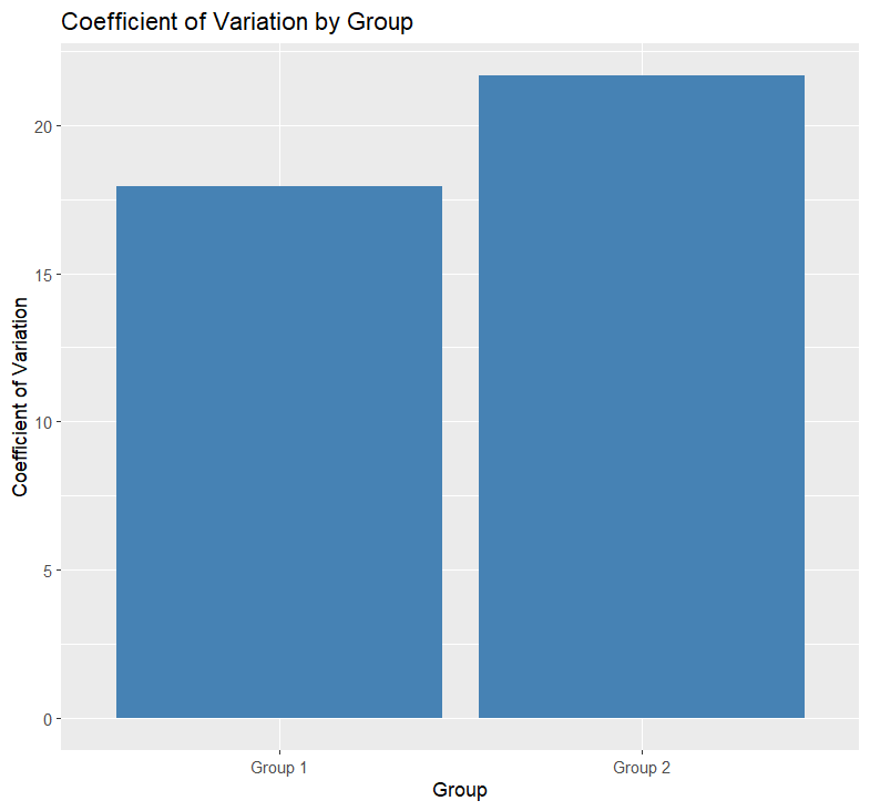
By executing this code, we will generate a bar plot that visualizes the coefficient of variation for each group. This allows us to compare the variability between different groups in a graphical manner, providing a clear visualization of the relative variability within each group.
Conclusion
In this post, you have learned about the coefficient of variation and how it measures the relative variability in a dataset. We explored its interpretation and significance in analyzing data. By calculating the coefficient of variation using base R and the dplyr package, you gained practical knowledge on applying this metric to your datasets.
We covered various scenarios, including calculating the coefficient of variation for individual variables by group and across multiple variables. You learned how to generate synthetic data, calculate the coefficient of variation using different methods, and visualize the results through plots. Additionally, we highlighted the importance of summarizing other statistical measures to understand your data comprehensively.
I hope you found this post informative and that it has expanded your knowledge of the coefficient of variation in R. If you have any suggestions or specific topics you would like me to cover in future posts, please comment below. Remember to share this post with others who may benefit from learning about the coefficient of variation. We can continue exploring and leveraging R’s robust data analysis and statistical measures capabilities.
R Tutorials
Here are some other tutorials related to R and tidyverse (e.g., dplyr and tidyr):
- Countif function in R with Base and dplyr
- How to Calculate Five-Number Summary Statistics in R
- Binning in R: Create Bins of Continuous Variables
- How to Add a Column to a Dataframe in R with tibble & dplyr
- How to Convert a List to a Dataframe in R – dplyr
- R Count the Number of Occurrences in a Column using dplyr
- How to Add an Empty Column to a Dataframe in R (with tibble)