In this short tutorial, you will learn how to find the five-number summary statistics in R. Specifically, in this post, we will calculate:
- Minimum
- Lower-hinge
- Median
- Upper-hinge
- Maximum
Now, we will also visualize the five-number summary statistics using a boxplot. First, we will learn how to calculate each of the five summary statistics and then how we can use one single function to get all of them directly.
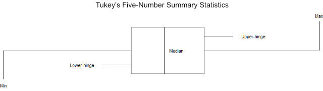
Table of Contents
- Requirements
- Find the Five-Number Summary Statistics in R: 6 Simple Steps
- Five-Nummer Summary Statistics Table
- Find Five-Number Summary Statistics in R with the fivenum() Function
- Visualizing the 5-Number Summary Statistics with a Boxplot
- Conclusion
- Other R Tutorials:
Requirements
To follow this R tutorial you will need to have readxl and ggplot2 installed. The easiest way to install these to r-packages is to use the install.packages() function:
install.packages(c("readxl", "ggplot"))Code language: R (r)Note, both these two packages are part of the Tidyverse. This means that you get them, as well as a lot of other packages when installing Tidyverse. For example, you can use packages such as dplyr to rename columns, remove columns in R, merge two columns, and select columns, as well.
Before getting to the 6 steps to finding the five-number summary statistics using R, we will get the answer to some questions.
As you may have understood, the five-number summary statistics are 1) the minimum, 2) the lower hinge, 3) the median, 4) the upper hinge, and 5) the maximum. The five-number summary is a quick way to explore your dataset.
The easiest way to find the five-number summary statistics in R is to use the fivenum() function. For example, if you have a vector of numbers called “A” you can run the following code: fivenum(A) to get the five-number summary.
Now that we know the five-number summary, we can learn the simple steps to calculate the five summary statistics.
Find the Five-Number Summary Statistics in R: 6 Simple Steps
In this section, we are ready to go through the six simple steps to calculate the five-number statistics using the R statistical environment. To recap: the first step is to import the dataset (e.g., from an xlsx file). Second, we calculate the min value, and then, in the third step, we get the lower hinge. In the fourth step, we get the median. In the fifth step, we get the upper hinge; in the sixth and final step, we get the max value.
Step 1: Import your Data
Here’s how to read a .xslx file in R using the readxl package:
library(readxl)
dataf <- read_excel("play_data.xlsx", sheet = "play_data",
                    col_types = c("skip", "numeric",
                                  "text","text", "numeric",
                                  "numeric", "numeric"))

head(dataf)Code language: JavaScript (javascript)
We can see that in this example dataset there’s only one column containing numerical data (i.e., the column RT). In the next step, we will take the minimum of this column. Note, it is also possible to create a matrix in R (in which you can store your data).
Step 2: Get the Minimum
Here’s how to get the minimum value in a column in R:
min.rt <- min(dataf$RT, na.rm = TRUE)Code language: PHP (php)Notice how we used the min() function with the dataframe and the column (i.e., RT) as the first argument. We set the second argument to TRUE because we have some missing values in the column. Finally, we used the $ operator in R to select a column. If we, on the other hand, were using dplyr we could use the select() function. That said, let’s move on and get the max value.
Step 3: Get the Lower-Hinge
Here’s how we get the lower hinge:
# Lower  Hinge:
RT <- sort(dataf$RT)
lower.rt <- RT[1:round(length(RT)/2)]
lower.h.rt <- median(lower.rt)Code language: PHP (php)
Notice, how we started by selecting only response times (i.e., the RT column) and sorted the values. Second, we get the lower part of the response times and then, we get the lower hinge by calculating the median of this vector.
Step 4: Calculate the Median
To calculate the median, we can use the median() function:
# Median
median.rt <- median(dataf$RT, na.rm = TRUE)Code language: PHP (php)
Again, we used the na.rmargument (TRUE) because there are some missing values in the dataset. Of course, if your data doesn’t have any missing values you can leave this argument out.
Step 5: Get the Upper-Hinge
Here’s how to get the upper hinge:
# Upper Hinge
RT <- sort(dataf$RT)
upper.rt <- RT[round((length(RT)/2)+1):length(RT)]
upper.h.rt <- median(upper.rt)Code language: PHP (php)
Similar to when we got the lower hinge, we first sorted the RT column. Then, we get the upper half and calculate its median of it.
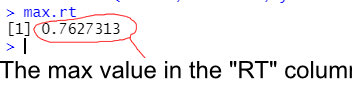
Step 6: Get the Maximum
We can get the maximum by using the max() function:
# Max
max.rt <- max(dataf$RT, na.rm = TRUE)Code language: PHP (php)
Again, we selected the RT column using the dollar sign operator and removed the missing values. Here’s the output:
Note, that the lower- and upper-hinge is the same as the first and third quartile when the sample size is odd. If this is the case, an easier way to get the lower- and upper-hinge is to use the quantile()function. In the example data above, however, we had an equal number of observations (leaving out the missing values). If you need to combine two variables, in your dataset, into one make sure to check this post out:
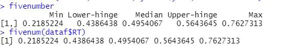
Five-Nummer Summary Statistics Table
In this section, we are going to put everything together so we get a somewhat nicer output:
fivenumber <- cbind(min.rt, lower.h.rt,
                    median.rt, upper.h.rt,
                    max.rt)
colnames(fivenumber) <- c("Min", "Lower-hinge",
                       "Median", "Upper-hinge", "Max")

fivenumberCode language: CSS (css)
As you can see in the above code chunk, we used the cbind() function to combine the different objects into one. Then, we give the combined object better column names. In the next section, we will see that there already is a function that can calculate the five-number statistics in R in one line of code, basically.

Find Five-Number Summary Statistics in R with the fivenum() Function
Here is how to find the five-number summary statistics in R with the fivenum() function:
# Five summary with R's fivenum()
 fivenum(dataf$RT)Code language: PHP (php)
Pretty simple. We just selected the column containing our data. Again, we used the $ operator to get the RT column and use the fivenum() function. Note that fivenum() function removes any missing values by default.
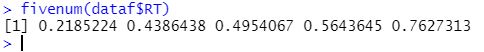
As you can see in the output above, we don’t get any column names but the five-number summary statistics are ordered as follows: min, lower-hinge, median, upper-hinge, and max. We can see that we get the same values as in the 6 step method:
In the next section, we will create a boxplot displaying the five-number summary statistics in R.
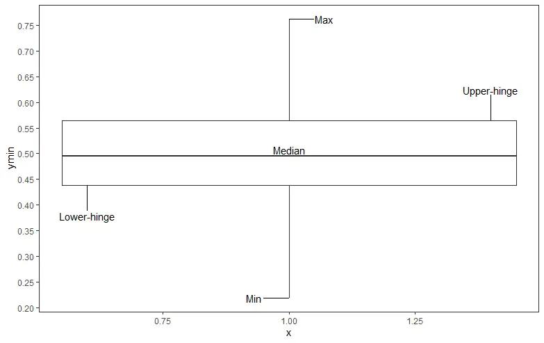
Visualizing the 5-Number Summary Statistics with a Boxplot
Here’s how we can visualize Tukey’s 5 number summary statistics in R using a boxplot:
library(ggplot2)

df <- data.frame(
  x = 1,
  ymin = fivenumber[1],
  Lower = fivenumber[2],
  Median = fivenumber[3],
  Upper = fivenumber[4],
  ymax = fivenumber[5]
)

ggplot(df, aes(x)) +
  geom_boxplot(aes(ymin=ymin, lower=Lower,
                   middle=Median, upper=Upper, ymax=ymax),
               stat = "identity") +
  scale_y_continuous(breaks=seq(0.2,0.8, 0.05)) +
  # Style the plot bit
  theme_bw() +
  theme(panel.grid.major = element_blank(),
       panel.grid.minor = element_blank()
  ) +
  # After this is just to annotate the plot and can be removed
  # Min
  geom_segment(aes(x = 1, y = ymin, xend = 0.95, yend = ymin), data = df) +
  annotate("text", x = 0.93, y = df$ymin, label = "Min") +
  # Lower-hinge
  geom_segment(aes(x = 0.60, y = Lower, xend = 0.60, yend = Lower-0.05), data = df) +
  annotate("text", x = 0.60, y = df$Lower-0.06, label = "Lower-hinge") +
  # Median
  annotate("text", x = 1, y = df$Median + .012, label = "Median") +
  # Upper-hinge
  geom_segment(aes(x = 1.40, y = Upper, xend = 1.40, yend = Upper+0.05), data = df) +
  annotate("text", x = 1.40, y = df$Upper+0.06, label = "Upper-hinge") +
  # Max
  geom_segment(aes(x = 1, y = ymax, xend = 1.05, yend = ymax), data = df) +
  annotate("text", x = 1.07, y = df$ymax, label = "Max") Code language: R (r)
We are not getting into details in the example above. However, we did create a dataframe from the first object we created and then we used ggplot() and ggplot_boxplot() to create the boxplot. Notice how we used the aes() function and set the different values found in the dataframe as arguments. Here ymin and ymax are the minimum and maximum values, respectively. Note we also changed the number of ticks on the y-axis. Here we used the seq() function to generate a sequence of numbers. The plot is somewhat styled and the code for drawing segments (lines) and adding text can be skipped, of course, if you want to visualize the five summary statistics in R.
More data visualization tutorials:
Conclusion
In this post, you have learned two ways to get the five summary statistics in R: 1) min, 2) lower-hinge, 3) median, 4) upper-hinge, and 5) max. In the first method, we calculated each of these summary statistics separately. Furthermore, we have also learned how to use the handy fivenum() function to get the same values. We created a boxplot from the five summary statistics in the final section. I hope you have learned something valuable. If you did, please link to the blog post in your projects and reports, share it on your social media accounts, and/or drop a comment below.
Other R Tutorials:
Here are some other tutorials that you may find useful:
- How to Take Absolute Value in R – vector, matrix, & data frame
- Learn How to Calculate Descriptive Statistics in R the Easy Way with dplyr
- How to Extract Year from Date in R with Examples
- Get the Absolute Value in R – from a vector, a matrix, & a data frame
- How to Rename Factor Levels in R using levels() and dplyr
- Learn How to Remove Duplicates in R – Rows and Columns (dplyr)
- How to Add a Column to a Dataframe in R with tibble & dplyr

Nice one!!! Thank you!
Hey Daniel,
Glad you liked it and that it (hopefully) helped you out,
Best,
Erik
you hav used max to find min, simple typo
Hey,
Thanks for your comment. I have now fixed this typo.