R Count the Number of Occurrences in a Column using dplyr

In this R tutorial, you will learn how to count the number of occurrences in a column. Sometimes, before starting to analyze your data,  it may be useful to know how many times a given value occurs in your variables. For example, when you have a limited set of possible values that you want to compare, In this case, you might want to know how many there are of each possible value before you carry out your analysis. Another example may be that you want to count the number of duplicate values in a column. Moreover, if we want an overview or information, let us say how many men and women you have in your data set. In this example, you must report the number of men and women in your research articles. Here, you will learn how to count observations in R.

Table of Contents

• Outline
• Prerequisites
  • Installing dplyr
• Importing Example Data
• How to Count the Number of Occurrences in R using table()
• How to Count the Number of Occurrences as well as Missing Values 
• Count How Many Times a Value Appears in a Column in R
• Calculating the Relative Frequencies of the Unique Values in R
• How to Count the Number of Times a Value Appears in a Column in R with dplyr
• Count the Relative Frequency of Factor Levels using dplyr
• How to create Bins when Counting Distinct Values 
• Conclusion
• R Tutorials

Outline

• Save

In this post, you will learn how to use the R function table() to count the number of occurrences in a column. Moreover, we will also use the function count() from the package dplyr. First, we start by installing dplyr and then we import example data from a CSV file. Second, we will begin looking at the table() function and how to use it to count distinct occurrences. Here, we will also look at how we can calculate the relative frequencies of factor levels.

Third, we will have a look at the count() function from dplyr and how to count the number of times a value appears in a column in R. Finally, we will also look at how we can calculate the proportion of factor/characters/values in a column. 

In the next section, you will learn how to install dplyr. Of course, if you prefer table(), you can jump to this section directly. 

Prerequisites

Here is what you need to know to follow this tutorial on counting unique values and occurrences in a column in R. First, ensure that you have R installed on your system. Using the latest stable version of R is recommended to benefit from its updated features and security enhancements. If you prefer a more user-friendly environment for R programming, consider installing RStudio, a popular integrated development environment (IDE) that provides a range of powerful tools and features.

To perform the operations covered in this tutorial, you must also install the dplyr package. This versatile package offers a wide range of data manipulation and analysis functions, making it an essential tool for working with data frames in R. If you still need to install the dplyr package, you can easily do so by running the command install.packages("dplyr") in your R console.

Installing dplyr

A basic understanding of R programming concepts and data manipulation will be helpful as you dive into this tutorial. Familiarity with functions, data frames, and working columns in R will enable you to follow along more effectively.

Additionally, it is a good practice to keep your R installation and packages up to date to ensure compatibility and take advantage of any bug fixes or performance improvements. Regularly updating R and its packages will ensure a smooth and efficient workflow. Here is how to install dplyr:

install.packages("dplyr")Code language: R (r)

Note that dplyr is part of the Tidyverse package, which can be installed. Installing the Tidyverse package will install several very handy and useful R packages. For example, we can use dplyr to remove columns, and remove duplicates in R. Moreover, we can use tibble to add a column to the dataframe in R. Finally, the package Haven can be used to read an SPSS file in R and to convert a matrix to a dataframe in R. For more examples, and R tutorials, see the end of the post.

In the upcoming sections, we will import example data to practice with and explore various methods for counting unique values and occurrences in a column in R. So, let us get started and harness the power of R for efficient data analysis and manipulation!

Importing Example Data

Before learning to use R to count the number of occurrences in a column, we need some data. For this tutorial, we will read data from a CSV file found online:

df <- read.csv('https://vincentarelbundock.github.io/Rdatasets/csv/carData/Arrests.csv')Code language: R (r)

This data contains details of a person who has been arrested, and in this tutorial, we will look at sex, checks, and age columns. First, the sex column classifies an individual’s gender as male or female. Second, the age is, of course, referring to an individual in the datasets age. Let us have a quick look at the dataset:

• Save

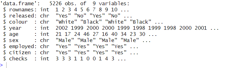
Using the str() function, we can see that we have 5226 observations across nine columns. Moreover, we can see the data type of the nine columns.

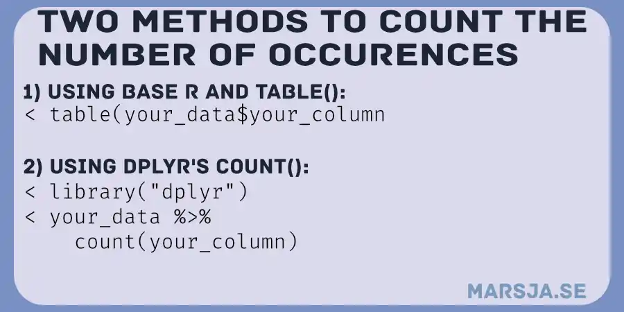
How to Count the Number of Occurrences in R using table()

Here is how to use the R function table() to count occurrences in a column:

table(df['sex'])Code language: R (r)

In the code chunk above, we counted the unique occurrences in the sex column using the table() function. By selecting the column sex with brackets (i.e., df[‘sex’]), we obtained the result. By using the table() function it allows us to analyze the distribution of unique values in the column. Here is the result:

• Save

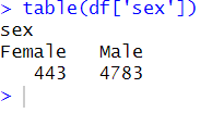
It is also possible to use $ in R to select a single column. Now, as you can see in the image above, the function returns the count of all unique values in the given column (‘sex’ in our case) in descending order without any null values. We see more men than women in the dataset by glancing at the above output. The results show us that the vast majority are men.

• Save

Note both of the examples above will remove missing values. This, of course, means that they will not be counted at all.  In some cases, however, we may also want to know how many missing values there are in a column. In the next section, we will therefore have a look at an argument that we can use (i.e., useNA) to count unique values and missing values in a column. First, however, we are going to add ten missing values to the column sex:

df_nan <- df
df_nan$sex[c(12, 24, 41, 44, 54, 66, 77, 79, 91, 101)] <- NaNCode language: R (r)

In the code above, we first used the column name (with the $ operator) and, then, used brackets to select rows. Finally, we used the NaN function to add the missing values to the selected rows. The next section will count the occurrences, including the ten missing values we added to the dataframe. Next, we will count observations in R, including missing values.

How to Count the Number of Occurrences as well as Missing Values

Here is a code snippet that you can use to get the number of unique values in a column as well as how many missing values:

df_nan <- df
df_nan$sex[c(12, 24, 41, 44, 54, 66, 77, 79, 91, 101)] <- NaN
table(df_nan$sex, useNA = "ifany")Code language: PHP (php)

In the code chunk above, we utilized the useNA argument to count the unique occurrences in the sex column, including missing values. By assigning NaN (Not a Number) to specific indices in the sex column of the dataframe, we introduced missing values. Importantly, with the useNA = "ifany" parameter, the table() function considered these missing values when counting unique occurrences in data.

• Save

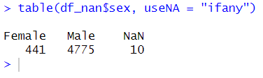
We already knew we had ten missing values in this column. Of course, when dealing with collected data, we may not know this and, thus, will let us know how many missing values there are in a specific column. In the next section, we will not count the number of times a value appears in a column in R. Next; we will instead count the relative frequencies of unique values in a column.

• Countif function in R with Base and dplyr

Count How Many Times a Value Appears in a Column in R

Here is how to count how many times a specific value appears in a column in R:

# Assuming 'df' is your dataframe and 'checks' is the column you want to count values in
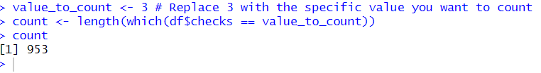
value_to_count <- 3 # Replace 3 with the specific value you want to count
count <- length(which(df$checks == value_to_count))Code language: PHP (php)

In the code chunk above, we count the number of occurrences of a specific value in a column called checks within the dataframe df. The value we want to count is specified as value_to_count, which is set to 3 in this example. We use the which() function to identify the positions in the checks column where the value equals 3. The length() function then gives us the total count of these positions, representing the number of times the value 3 appears in the checks column. The result is stored in the variable count. This code allows us to efficiently determine how frequently the specified value occurs in the given column of the dataframe.

• Save

Calculating the Relative Frequencies of the Unique Values in R

Another thing we can do, now that we know how to count unique values in a column in R’s dataframe is to calculate the relative frequencies of unique values. Here’s how we can calculate the relative frequencies of men and women in the dataset:

table(df$sex)/length(df$sex)Code language: PHP (php)

In the code chunk above, we used the table() function as in the first example.  We added something to get the relative frequencies of the factors (i.e., men and women). In the example above, we used the length() function to get the total observations. We used this to calculate the relative frequency. This may be useful if we want to count the occurrences and want to know, e.g., what percentage of the male and female sample.

How to Count the Number of Times a Value Appears in a Column in R with dplyr

Here is how we can use R to count the number of occurrences in a column using the package dplyr:

library(dplyr)

# Assuming 'df' is your dataframe and 'sex' is the column you want to count unique values in
df %>% 
  count(sex)Code language: R (r)

• Save

In the example above, we used the %>% operator, which enables us to use the count() function to get this beautiful output. Now, as you can see, when we are counting the number of times a value appears in a column in R using dplyr we get a different output compared to when using table(). For another great operator, see the post about how to use the %in% operator in R.

In the next section, we will count the relative frequencies of factor levels. Again, we will use dplyr but this time, we will use group_by(), summarise(), and mutate().

Count the Relative Frequency of Factor Levels using dplyr

In this example, we will use three R functions (i.e., from the dplyr package). First, we use the piping operator again and then group the data by a column. After we have grouped the data we count the unique occurrences in the column, we have selected. Finally, we are calculating the frequency of factor levels:

df %>%
  group_by(sex) %>%
  summarise(n = n()) %>%
  mutate(Freq = n/sum(n))Code language: R (r)

Using the code above, we get two columns. In the code chunk above, we grouped the data by the column containing gender information. We then summarized the data. Using the n() function, we got the number of observations of each value. Finally, we calculated a new variable called “Freq”. Here is where we calculate the frequencies. This gives us another nice output. Let us have a look at the output:

• Save

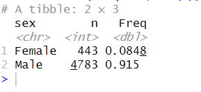
As you can see in the output, above, we get two columns. This is because we added a new column to the summarized data: the frequencies. Of course, counting a column, such as age, as we did in the previous example, would not provide any useful information. The next section will use the R package dplyr to count unique occurrences in a column. 

There are 53 unique values of age data, a mean of 23.84 and a standard deviation of 8.31. Therefore, counting the unique values of the age column would produce a lot of headaches. In the next example, we will look at how to count age but get a readable output by binning. This is useful if we want to count, e.g., even more continuous data. 

How to create Bins when Counting Distinct Values

As previously mentioned, we can create bins and count the number of occurrences in each of these bins. Here’s an example code in which we get five bins:

df %>%
  group_by(group = cut(age, breaks = seq(0, max(age), 11))) %>%
  summarise(n = n())Code language: R (r)

In the code chunk above, we used the group_by() function, again (of course, after the %>% operator). In this function, we also created the groups (i.e., the bins). Here we used the seq() function that can be used to generate a sequence of numbers in R. Finally, we used the summarise() function to get the number of occurrences in the column, binned. Here’s the output:

• Save

For each bin, the range of age values is the same: 11 years. One contains ages from 11 to 22. The next bin has ages from 22 to 33.  However, we also see a different number of people in each age range. This enables us to see that most people arrested are under 22. Now, this makes sense in this case, right? 

• Binning in R: Create Bins of Continuous Variables

Conclusion

In this post, you have learned how to count the number of occurrences in R using various methods and functions. We explored the table() function to count unique values in a column and calculate their relative frequencies. We also discussed handling missing values and including them in the count using the useNA argument.

• Save

Furthermore, we covered the dplyr package, which provides powerful tools for counting occurrences and manipulating data. With dplyr, you discovered how to count the times a specific value appears in a column and calculate the relative frequency of factor levels.

• Save

We also learned how to create bins (i.e., counting distinct values). This allows us to more comprehensive data distribution analysis. Throughout the post, we looked at code examples and explanations to help you understand and apply these counting techniques in your projects.

By learning these methods, you will get the skills to efficiently count occurrences, calculate relative frequencies, and gain insights from your data. These counting techniques will prove invaluable if you need to analyze, e.g., survey responses, track product sales, or explore any other dataset.

Remember to update your R installation and have the necessary packages, such as dplyr, installed. With these tools, you can count the number of occurrences and explore the distribution of values in your data. Make sure you share this post on your social media accounts so, e.g., your colleagues can learn. Leave a comment below!

R Tutorials

Here are a bunch of other tutorials you might find useful:

• How to Do the Brown-Forsythe Test in R: A Step-By-Step Example
• Select Columns in R by Name, Index, Letters, & Certain Words with dplyr
• How to Calculate Five-Number Summary Statistics in R
• Probit Regression in R: Interpretation & Examples
• How to Concatenate Two Columns (or More) in R – stringr, tidyr
• Correlation in R: Coefficients, Visualizations, & Matrix Analysis
• How to Create a Violin plot in R with ggplot2 and Customize it
• Master or in R: A Comprehensive Guide to the Operator