Probit Regression in R: Interpretation & Examples

This blog post will teach us how to use probit regression in R, a statistical modeling technique for analyzing binary response variables. Probit regression can be useful when the outcome variable is dichotomous. That is when the outcome variable takes only two possible values, such as “success” or “failure,” “yes” or “no,” or “tinnitus” or “no tinnitus.”

We will start by exploring examples of when to use probit regression in R. Then, we will look at other alternatives and compare them to probit regression. We will also provide an example dataset that we can use to illustrate how to perform probit regression in R.

Once we have a dataset, we will dive into the syntax of building a probit model in R, explaining each step. We will also provide a complete example of probit regression in R to see how it fits together.

Probit Model
Examples of When to use Probit Regression in R
Other Alternatives
Example Data for Probit Regression in R
Probit Model in R
Probit Regression in R Examples
Visualize a Probit Model in R
Summary
Resources

Finally, we will learn how to visualize a probit model using ggplot2, a powerful data visualization package in R. By creating a predicted probability plot, we can see the relationship between our predictor variables and the probability of the outcome variable.

Probit Model

We can use probit regression in R to model the relationship between a binary variable and one or more predictor variables. Note that a binary variable takes on one of two possible values, such as the presence or absence of a particular characteristic. The main goal of probit regression is to estimate the probability that the binary response variable is equal to 1 (as opposed to 0) as a function of the predictor variables.

Probit regression is based on the assumption that the relationship between the predictors and the probability of the response variable can be modeled using the cumulative distribution function (CDF) of a normal distribution. In other words, probit regression assumes that the probability of the response variable being equal to 1 can be modeled using a normal probability density function and that the values of the predictor variables determine the mean and standard deviation of the distribution.

probit regression in R: predicted probabilities visualized using gplot2 — Predicted Probabilities of Hypothetical Data

In a recent post, you can learn how to make a plot prediction in R using ggplot2. This plot type can be used for linear and non-linear regression models. Remember to test for normality of the residuals or create a residual plot.

Examples of When to use Probit Regression in R

There are several examples of how probit regression can be applied in psychology and hearing science:

In a study investigating the effect of a new treatment on depression, researchers may use probit regression. Here, we can use it to model the relationship between the treatment (predictor variable) and the likelihood of a patient experiencing reduced depression symptoms (binary response variable).
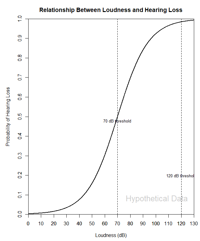
Researchers may use probit regression in a study examining the relationship between noise exposure and the likelihood of hearing loss. They can use it to model the relationship between the loudness of sounds (predictor variable) and the likelihood of a participant experiencing hearing loss (binary response variable). If we conducted such a study, it could help determine the threshold at which loud sounds can cause hearing damage, which can be used to set occupational safety standards for workers in noisy environments.
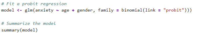
In a study investigating the effect of age and gender on the likelihood of experiencing anxiety, researchers may use probit regression to model the relationship between age, gender (predictor variables), and the likelihood of experiencing anxiety (binary response variable).

Other Alternatives

We can use several alternative analysis methods for data like the ones described in examples 1-3. Here are a few examples:

Logistic Regression: Logistic regression is a generalized linear model for binary outcomes. It is similar to probit regression, which models the relationship between a binary outcome variable and one or more predictor variables. However, logistic regression uses a different link function (the logistic function) to model the relationship between the predictor variables and the probability of the binary outcome.
Generalized Estimating Equations (GEE): GEE is a method for analyzing data with correlated outcomes, such as repeated measures data or clustered data. GEE allows for the estimation of regression coefficients adjusted for within-subject or within-cluster correlations, which can improve the estimates’ accuracy and the statistical inference’s validity.
Mixed-effects models: Mixed-effects models are regression models that analyze data with fixed and random effects. They are handy for analyzing nested or hierarchical data structures, such as repeated measures data or clustered data. Mixed-effects models can also be used to analyze longitudinal data or data with missing values.
Bayesian methods: Bayesian methods are a family of statistical methods based on Bayes’ theorem. They are particularly useful for analyzing complex data structures and models. They allow for incorporating prior knowledge and uncertainty into the analysis. Bayesian methods can analyze data with binary outcomes, repeated measures, clustered, and longitudinal data.
Machine learning methods: Machine learning methods are a family of computational methods used to build predictive models from data. They are particularly useful for analyzing large and complex data sets, as they can handle many predictor variables and non-linear relationships between the predictor variables and the outcome variable. Some common machine-learning methods include decision trees, random forests, and support vector machines.

The choice of analysis method will depend on the specific research question, the data type, and the different techniques’ assumptions. It is important to consider each method’s strengths and limitations carefully and choose the most appropriate method for the research question.

Example Data for Probit Regression in R

We will generate two pieces of example data: one with continuous variables and one with a categorical variable. Note that you are free to use your data, and the data is not related to any actual studies.

Example Data 1: Two Continuous Variables

Suppose that we are interested in the predictors of hearing aid use. We have a dataset with 500 observations with two continuous variables: age, the experience of hearing aids, and the binary response variable hearing aid use. We assume a relationship between the predictor variables and the binary response variable.

# Set coefficients
beta0 <- -0.5
beta1 <- 1.5
beta2 <- 2.5

# Simulate data
n <- 500

age <- rnorm(n, 50, 10)
experience <- rnorm(n, 15, 3)

x1 <- scale(age) 
x2 <- scale(experience)
eta <- beta0 + beta1*x1 + beta2*x2
eta <- eta + rnorm(n, 0, 0.1)
hau <- rbinom(n, 1, pnorm(eta))

# Create dataframe
df1 <- data.frame(hau, age=age, experience=experience)Code language: R (r)

Here are some tutorials that you may find useful for generating dataframes in R:

Example Data 2: Continuous & Categorical Variables

Suppose we have collected data from 500 participants with hearing loss to investigate the relationship between hearing loss and tinnitus. In the study, we also collected audiogram data and calculated the pure-tone audiogram (PTA) at four frequencies (e.g., 500 Hz, 1000 Hz, 2000 Hz, and 4000 Hz). Additionally, we obtained demographic information, including the gender of each participant. Using this data, we want to investigate whether there is an association between PTA4 and the presence of tinnitus while also considering gender. Finally, we collected self-reported tinnitus symptoms on a binary scale (yes or no). Here, we simulate this hypothetical data:

# Set seample size
samp_n <- 500

# Set random seed for reproducibility
set.seed(123)

# Generate PTA4 values
PTA4 <- rnorm(samp_n, mean = 50, sd = 10)

# Generate gender values
gender <- rbinom(samp_n, size = 1, prob = 0.5)

# Calculate probability of tinnitus based on coefficients
prob_tinnitus <- pnorm(0.890118 - 0.015338*PTA4 - 0.584865*gender)

# Generate tinnitus values based on probabilities
tinnitus <- rbinom(samp_n, size = 1, prob = prob_tinnitus)

# Create dataframe
df2 <- data.frame(PTA4 = PTA4, 
                 gender = ifelse(gender == 1, "Male", "Female"),
                 tinnitus = tinnitus)Code language: R (r)

Although not a requirement, it may be easier to transform your data from wide to long in R using tidyr before analyzing using the glm() function.

Descriptive Statistics

First, before carrying out the probit regression, we can calculate descriptive statistics in R using dplyr:

library(dplyr)
df2 %>% group_by(gender) %>% 
  summarise("Mean Tinnitus" = mean(tinnitus),
            "SD Tinnitus" = sd(tinnitus),
            "Mean PTA4" = mean(PTA4),
            "SD PTA4" = sd(PTA4)Code language: JavaScript (javascript)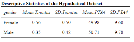

Probit Model in R

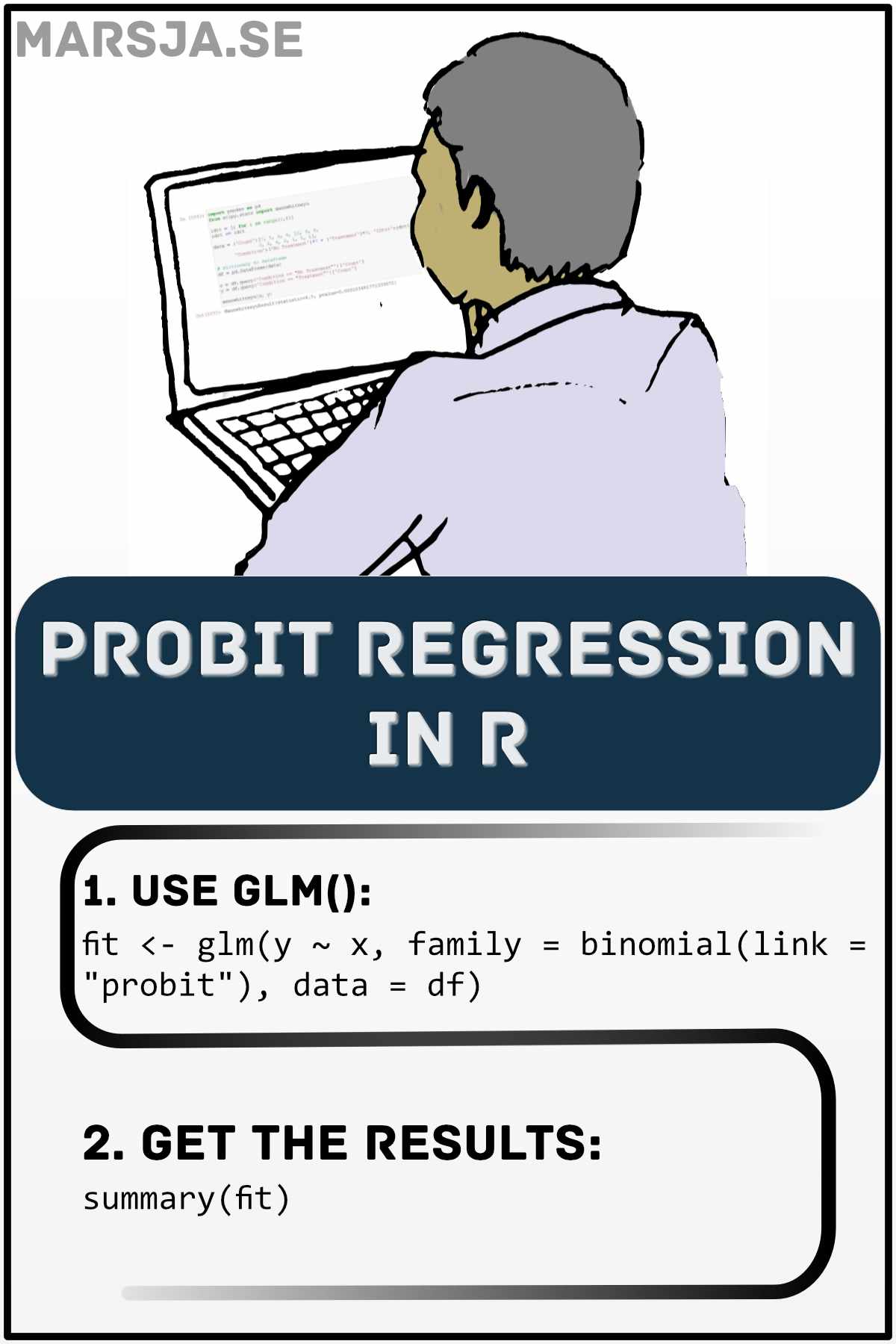
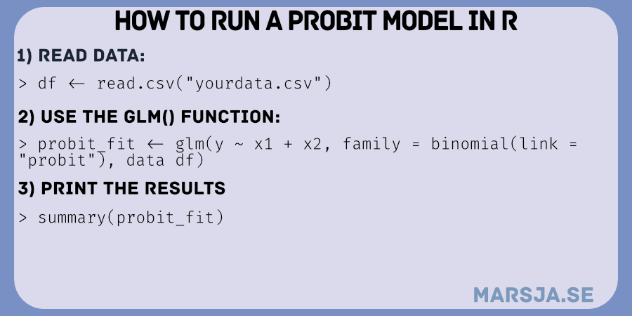
To carry out probit regression in R, we can use the following steps:

Define the formula for the regression model in the glm() function. The formula specifies the binary response variable and one or more predictor variables.
Set the family argument in the glm() function to binomial(link = "probit") to specify that the probit link function should be used.
Fit the model by calling the glm() function with the formula and data as arguments.
Use the summary() function to print the results.

Probit Regression in R Examples

This section will explore how to perform probit regression in R with continuous and categorical predictor variables.

Probit Regression in R with Continuous Variables

Here is how we carry out a probit regression in R with continuous variables:

# Run probit model
expage_model<- glm(hau ~ experience + age, family = binomial(link = "probit"), data = df1)

# View model summary
summary(expage_model)Code language: HTML, XML (xml)

In the code chunk above, we run a probit regression model in R with experience and age as predictors to explain the probability of hau (i.e., hearing aid use). We use the glm() function to estimate the model with the family argument set to “binomial” and the link argument set to “probit” to indicate that we are estimating a probit regression model. The data argument specifies the data frame where the variables are located.

Probit Regression in R with a Categorical Variable

Here is how we run a probit model in R with a continuous and a categorical variable:

tinnitus_probit <- glm(tinnitus ~ PTA4 + gender,  family = binomial(link = "probit"), 
                data = df2)Code language: R (r)

In the code chunk above, we use the glm() function in R to conduct probit regression. We use the formula argument to specify the model we want to fit. In this case, we fit a model with tinnitus as the binary response variable and PTA4 and gender as the predictor variables. Again, we use the tilde (~) symbol to separate the response and predictor variables.

Importantly, we use the family argument to specify the type of response variable we are working with. In this case, we use the binomial family because tinnitus is a binary variable. The link argument is used to specify the type of link function we want to use. In this case, we use the probit link function because we are interested in modeling the probability of tinnitus using a normal distribution.

Finally, the data argument is used to specify the dataset we want to use for the analysis. In this case, we are using the df dataset we created earlier. Note that we do not have to create a dummy variable in R of the gender variable, the glm()function will handle this for us.

How to Interpret Probit Regression in R

To print the results, we can use the summary()function:

## model summary
summary(tinnitus_probit)Code language: PHP (php)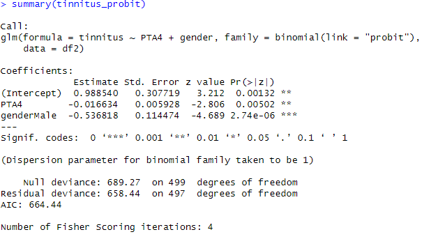

From the output above, we can see that the Intercept (or baseline probability) is -0.69806. This means that the predicted probability of having tinnitus is 0.498, or close to 50% when PTA4 and gender are both 0 (i.e., the reference group).

Moreover, we can see that the PTA4 coefficient is 0.06830. Here we can infer that for each unit increase in PTA4, the predicted probability of having tinnitus increases by a factor of exp(0.06830) = 1.070, or about 7%. This effect is statistically significant with a p-value of 1.17e-08.

Finally, we can see that the genderMale coefficient is -0.56991. This means that the predicted probability of tinnitus is exp(-0.56991) = 0.566, or about 57%, lower for males than females. This effect is also statistically significant, with a p-value of 0.0039.

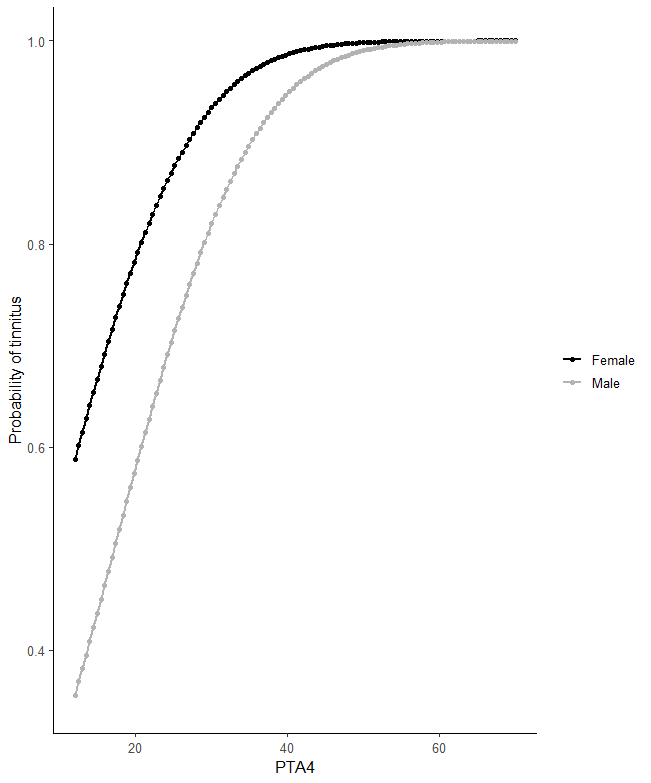
Visualize a Probit Model in R

One way to visualize a probit model is to create a predicted probability plot. This plot shows the relationship between the predictor variable(s) and the probability of the outcome variable.

Here is how we can use ggplot2 in R:

library(ggplot2)

# Generate predicted probabilities
df2$predicted_prob <- predict(tinnitus_probit, type="response")

# Create a predicted probability plot
ggplot(df2, aes(x=PTA4, y=predicted_prob, color=gender)) +
    geom_point() +
    geom_smooth(method="glm", method.args=list(family=binomial(link="probit")), se=F) +
    labs(x="PTA4", y="Probability of tinnitus") +
    scale_color_manual(values=c("blue", "red"), labels=c("Female", "Male")) +
    theme_bw()Code language: R (r)

In the code chunk above, we first load the ggplot2 library. Then, we use the predict function to generate predicted probabilities based on our probit regression model. These probabilities are added to the original dataframe as a new column called “predicted_prob”.

Next, we create a scatter plot using ggplot, where the x-axis represents the PTA4 and the y-axis represents the predicted probability of tinnitus. We color the points based on gender using the “color” aesthetic.

To add a smooth line to the scatter plot, we use the “geom_smooth” function. Here we used the “method” argument set to “glm” to indicate that we want to fit a generalized linear model. We specify the family as binomial with a probit link function using the “method.args” argument. We set “se” to “F” to remove the standard error shading.

Finally, we add x and y-axis labels using “labs” and set the colors for the two genders using “scale_color_manual”. We also apply a black-and-white theme using “theme_bw”. Here is the resulting plot:

Note that you can check the fit of your model by calculating the total sum of squares or the sum of squared errors in R.

Summary

In this blog post, we have learned about probit regression, a type of logistic regression used to model binary outcomes. We have explored examples of when to use probit regression in hearing science and audiology. We have also looked at alternative models for binary outcomes, such as logistic regression and discriminant function analysis.

To illustrate how to perform probit regression in R, we have generated example data and provided the R syntax for running the model. We have also demonstrated how to visualize the model using the ggplot2 package.

Furthermore, we have discussed how to interpret the results of a probit regression analysis. Here we looked at the deviance residuals, but coefficients and significance codes, in particular.

In conclusion, probit regression is a useful tool for modeling binary outcomes with continuous predictors in R. By using probit regression, we can gain insights into the relationship between the predictor variables and the binary outcome. Visualizing the model can help us better understand and communicate the results to others.

Resources

Here are some tutorials that you will likely find helpful: