In this blog post, you will learn how to test for the normality of residuals in R. Testing the normality of residuals is a step in data analysis. It helps determine if the residuals follow a normal distribution, which is important in many fields, including data science and psychology. Approximately normal residuals allow for powerful parametric tests, while non-normal residuals can sometimes lead to inaccurate results and false conclusions.
Testing for normality in R can be done using various methods. One of the most commonly used tests is the Shapiro-Wilks test. This test tests the null hypothesis that a sample is drawn from a normal distribution. Another popular test is the Anderson-Darling test, which is more sensitive to deviations from normality in the distribution’s tails. Additionally, the Kolmogorov-Smirnov test can be used to test for normality. The Kolmogorov-Smirnov test compares the sample distribution to a normal one with the same mean and standard deviation. In addition to using various normality tests, it’s important to incorporate data visualization techniques to assess normality.
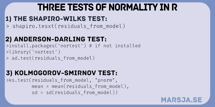
This blog post will provide examples of normality testing in data science and psychology and explain that the normality of residuals is crucial. We will also cover the three methods for testing the normality of residuals in R: the Shapiro-Wilks, Anderson-Darling, and Kolmogorov-Smirnov tests. We will explore how to interpret the results of each test and guide how to report the results according to APA 7. Having approximately normal residuals is essential for powerful parametric tests, while non-normal residuals can lead to inaccurate results and false conclusions.
Table of Contents
- Normality Testing: Why it’s Important and How to Test for Normality
- Examples of Normality in Data Science and Psychology
- Testing for Normality
- Anderson-Darling Test
- Parametric Tests and Normality
- Normality Violated
- Requirements
- Example Data
- How to Test for Normality in R: Three Methods
- Shapiro-Wilks Test for Normality
- Interpreting the Shapiro-Wilks Test
- Reporting the Shapiro-Wilks Test for Normality: APA 7
- Anderson-Darling Test for Normality
- Non-Normal Data
- Normal Data
- Interpret the Anderson-Darling Test for Normality
- Report the Anderson-Darling Test: APA 7
- Kolmogorov-Smirnov Test for Normality
- Interpreting the Kolmogorov-Smirnov Test
- How to Report the Kolmogorov-Smirnov Test: APA 7
- Dealing with Non-normal Data
- Additional Approaches
- Conclusion: Test for Normality in R
- Resources
Normality Testing: Why it’s Important and How to Test for Normality
Normality is a fundamental concept in statistics that refers to the distribution of a data set (residuals in our case). A normal distribution, also known as a Gaussian distribution, is a bell-shaped curve that is symmetric around the mean. In other words, the data is evenly distributed around the center of the distribution, with most values close to the mean and fewer values further away.
Normality can be important in some cases because common statistical tests, such as t-tests and ANOVA, assume the residuals are normally distributed. If the residuals are not normally distributed, these tests may not be valid and can lead to incorrect conclusions. Therefore, we can test for normality before using these tests.
Examples of Normality in Data Science and Psychology
Normality is a concept that is relevant to many fields, including data science and psychology. In data science, normality is important for many tasks, such as regression analysis and machine learning algorithms. For example, in linear regression, normality is a key assumption of the model. In this case, violations of normality can lead to biased or inconsistent estimates of the regression coefficients.
In psychology, normality is often used to describe the distribution of scores on psychological tests. For example, intelligence tests are designed to have a normal distribution, with most people scoring around the mean and fewer people scoring at the extremes. Normality is also important in hypothesis testing in psychology. Many statistical tests in psychology, such as t-tests and ANOVA, assume that the residuals are normally distributed. In some cases, violations of normality can lead to incorrect conclusions about the significance of the results.
Testing for Normality
There are several methods for testing normality, including graphical methods and formal statistical tests. Graphical methods include histograms, box plots, and normal probability plots. We can use these methods to visually inspect the data and assess whether it follows a normal distribution.
Formal statistical tests for normality include the Shapiro-Wilk test, the Anderson-Darling test, and the Kolmogorov-Smirnov test. These tests use different statistics to assess whether the data (e.g., residuals) deviates significantly from a normal distribution. All the tests should be used with caution and not on their own. In many cases, residual plots such as normal Q-Q plots, histograms, and residuals vs. fitted plots are more informative.
Shapiro-Wilks Test
The Shapiro-Wilks test is commonly used to check for normality in a dataset. It tests the null hypothesis that a sample comes from a normally distributed population. The test is based on the sample data and computes a test statistic that compares the observed distribution of the sample with the expected normal distribution.
The Shapiro-Wilks test is considered one of the most powerful normality tests. This means that it has a high ability to detect deviations from normality when they exist. However, the test is sensitive to sample size. It may detect deviations from normality in larger samples, even if the deviations are small and unlikely to affect the validity of parametric tests.
One can use statistical software such as R or Python to perform the Shapiro-Wilks test. The test returns a p-value that can be compared to a significance level to determine whether the null hypothesis should be rejected. A small p-value indicates that the null hypothesis should be rejected, meaning the sample is not normally distributed.
It is important to note that normality tests, including the Shapiro-Wilks test, should not be used as the sole criterion for determining whether to use parametric or non-parametric tests. Rather, they should be used with other factors such as the sample size, research question, and data analysis type.
Anderson-Darling Test
The Anderson-Darling test is another widely used normality test that can be used to check if a sample comes from a normally distributed population. The test is more sensitive to deviations from normality in the distribution’s tails, making it useful when it is important to ensure that the sample data is not just close to normal, but also has a similar shape.
Similar to the Shapiro-Wilks test, the Anderson-Darling test is based on the sample data and computes a test statistic that compares the observed distribution of the sample with the expected normal distribution. The test returns a p-value that can be compared to a significance level to determine whether the null hypothesis should be rejected.
The Anderson-Darling test has some advantages over other normality tests, including its ability to detect deviations from normality in smaller sample sizes and deviations in the distribution’s tails. However, it can be less powerful than the Shapiro-Wilks test in certain situations.
To perform the Anderson-Darling test, one can use statistical software such as R or Python. The test is widely available in most statistical software packages, making it easily accessible to researchers and analysts.
It is important to note that normality tests, including the Anderson-Darling test, should not be used as the sole criterion for determining whether to use parametric or non-parametric tests. Rather, they should be used with factors such as the sample size, research question, and data analysis type.
The Kolmogorov-Smirnov Test for Normality
The Kolmogorov-Smirnov test is a statistical test used to check if a sample comes from a known distribution. Moreover, the test is non-parametric and can be used to check for normality and other distributions.
The test is based on the maximum difference between the sample’s cumulative distribution function (CDF) and the expected CDF of the tested distribution. The test statistic is called the Kolmogorov-Smirnov statistic and is used to determine if the null hypothesis should be rejected.
To perform the Kolmogorov-Smirnov test, one can use statistical software such as R or Python. The test returns a p-value that can be compared to a significance level to determine whether the null hypothesis should be rejected.
The Kolmogorov-Smirnov test is widely used in many fields, including finance, biology, and engineering. It is particularly useful when the sample size is small, or the underlying distribution is unknown.
However, like other normality tests, the Kolmogorov-Smirnov test should not be used as the sole criterion for determining whether to use parametric or non-parametric tests. Instead, it should be used with factors such as the sample size, research question, and data analysis type.
Parametric Tests and Normality
Parametric tests, such as t-tests and ANOVA, assume the model’s residual follows a normal distribution. However, violations of normality assumptions may be a minor concern for ANOVA and other parametric tests (e.g., regression, t-tests). The central limit theorem indicates that the distribution of means of samples taken from a population will approach normality, even if the original population distribution is not normal. This means that the ANOVA results may still be reliable even if the residuals are not normally distributed, especially when the sample sizes are large. Nevertheless, if the sample sizes are small or the deviations from normality are severe, non-parametric tests may be more appropriate.
Normality Violated
If normality tests indicate that the residuals do not follow a normal distribution, several alternatives should be considered. These alternatives are non-parametric tests, which do not make any assumptions about the underlying distribution of the data. Non-parametric tests are often used when the assumptions of parametric tests, such as normality, are not met.
Here are some examples of non-parametric tests:
- Mann-Whitney U test is a non-parametric alternative to the t-test used to compare two independent samples. It does not assume that the data follows a normal distribution, but it does assume that the two groups have the same shape.
- Wilcoxon signed-rank test is a non-parametric alternative to the paired t-test to compare two related samples. It also does not assume that the residuals follow a normal distribution.
- The Kruskal-Wallis test is a non-parametric alternative to the ANOVA to compare three or more independent groups. It does not assume that the residuals follow a normal distribution, but it does assume that the variances of the groups are equal.
- Friedman test: This test is a non-parametric alternative to the repeated-measures ANOVA, used to compare three or more related samples. It also does not assume that the residuals follow a normal distribution.
Non-parametric tests are generally less powerful than their parametric counterparts, meaning they require a larger sample size to achieve the same level of statistical significance. However, they are more robust to violations of assumptions, such as normality, and are therefore often used when the data does not meet the assumptions of parametric tests. It is important to note that non-parametric tests also have their assumptions, such as independence, and should be chosen based on the research question and the data being analyzed.
Requirements
It would be best if you had basic statistics and data analysis knowledge to follow this blog post. Understanding normal distributions and statistical tests, such as t-tests and ANOVA, would be helpful.
You will also need access to R programming language and RStudio. The code in this blog post is written in R, so you must have R installed on your computer. Additionally, we used several R packages, including “nortest,” and “dplyr,” so you will need to have these packages installed as well.
To install an R package, you can use the following code in your R console:
install.packages("package_name")Code language: R (r)In our case, we can run this code install.packages(c("dplyr", "nortest")).
Example Data
Here is some example data to use to practice testing for normality in R:
library(dplyr)
# For reproducibility
set.seed(20230410)
# Sample size
n_nh <- 100
n_hi <- 100
# Generate normally distributed variable (working memory capacity)
wm_capacity_nh <- rnorm(n_nh, mean = 50, sd = 10)
wm_capacity_hi <- rnorm(n_hi, mean = 45, sd = 10)
wm_capacity <- c(wm_capacity_nh, wm_capacity_hi)
# Generate non-normal variable (reaction time)
reaction_time_nh <- rlnorm(n_nh, meanlog = 4, sdlog = 1)
reaction_time_hi <- rlnorm(n_hi, meanlog = 3.9, sdlog = 1)
reaction_time <- c(reaction_time_nh, reaction_time_hi)
# Create categorical variable (hearing status)
hearing_status <- rep(c("Normal", "Hearing loss"), each = 50)
# Combine variables into a data frame
psych_data <- data.frame(Working_Memory_Capacity = wm_capacity,
Reaction_Time = reaction_time,
Hearing_Status = hearing_status)
# Recode categorical variable as a factor
psych_data <- psych_data %>%
mutate(Hearing_Status = recode_factor(Hearing_Status,
"Normal" = "1",
"Hearing loss" = "2"))
# Rename variables
psych_data <- psych_data %>%
rename(WMC = Working_Memory_Capacity,
RT = Reaction_Time,
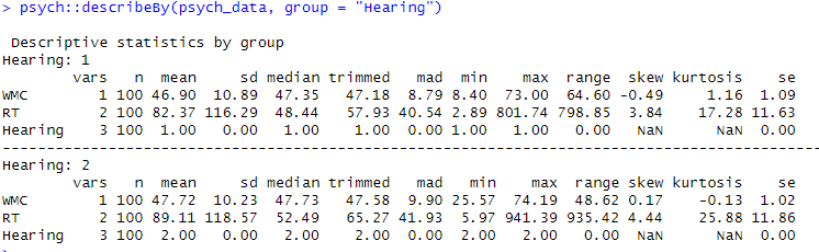
Hearing = Hearing_Status)Code language: PHP (php)In the code chunk above, we first load the dplyr library for data manipulation.
Next, we use the rnorm function to generate 50 random numbers from a normal distribution with a mean of 50 and standard deviation of 10 and store them in the wm_capacity_nh variable. Note that we do the same for the wm_capacity_hi. Finally, we create a wm_capacity variable by combining these two vectors.
We then use the rlnorm function to generate 100 random numbers from a lognormal distribution with a meanlog of 4 and sdlog of 1 and store them in the reaction_time_nh variable (almost the same for the reaction_time_hi)
To create a categorical variable, we use the rep function to repeat the values “Normal” and “Hearing loss” each 50 times and store them in the hearing_status variable.
We then combine the three variables into a data frame called psych_data using the data.frame function.
To recode the hearing_status variable as a factor with levels “1” and “2” corresponding to “Normal” and “Hearing loss”, respectively, we use the mutate function from dplyr along with the recode_factor function. Of course, recoding the factor levels in R might not be useful, and you can skip this step.
Finally, we use the rename function to rename the variables to “WMC” and “RT” for Working Memory Capacity and Reaction Time, respectively, and “Hearing” for the categorical variable.
How to Test for Normality in R: Three Methods
In this section, we will check for normality in R using three different methods. These methods are the Shapiro-Wilks test, the Anderson-Darling test, and the Kolmogorov-Smirnov test. Each of these tests provides a way to assess whether a sample of data comes from a normal distribution. Using these tests, we can determine if assumptions of normality are met for parametric statistical tests, such as t-tests or ANOVA. In the following sections, we will describe these tests in more detail and demonstrate how to perform them in R.
Shapiro-Wilks Test for Normality
To perform a Shapiro-Wilks test for normality in R on the psych_data data frame we created earlier, we can use the shapiro.test function.
Non-Normal Data
Here is an example code that performs a Shapiro-Wilks test on the RT variable and outputs the test results:
# First we carry out an ANOVA:
aov.fit.rt <- aov(RT  ~ Hearing, data = psych_data)

# Perform Shapiro-Wilks test dependent variable RT
shapiro.test(aov.fit.rt$residuals)Code language: PHP (php)
In the code chunk above, an ANOVA is performed using the psych_data dataset. The ANOVA model is specified with RT as the dependent variable and Hearing as the independent variable. The results are stored in the object aov.fit.
The following line of code uses the Shapiro-Wilk test to test for the normality of the residuals. The residuals are extracted from the ANOVA object using $residuals.
Normal Data
Here is an example code that runs the Shapiro-Wilks test for normality on the WMC variable:
aov.fif.wmc <- aov(WMC  ~ Hearing, data = psych_data)

# Perform Shapiro-Wilks test dependent variable WMC
shapiro.test(aov.fif.wmc$residuals)Code language: PHP (php)
In the code chunk above, we perform an ANOVA using the psych_data dataset. The ANOVA model is specified with WMC as the dependent variable and Hearing as the independent variable, just like in the case of RT above. The results are stored in the object aov.fif.wmc.
In the final line of code, we use the Shapiro-Wilk test to test for normality of the residuals from the ANOVA object aov.fif.wmc.
Interpreting the Shapiro-Wilks Test
Interpreting the results from a Shapiro-Wilks test conducted in R is pretty straightforward. For the model including the reaction time variable, the p-value is less than 0.05 (for both groups), and we reject the null hypothesis that the residuals are normally distributed.
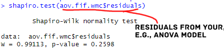
On the other hand, for the model including working memory capacity as the dependent variable, the p-value is greater than 0.05 (for both groups). We fail to reject the null hypothesis that the residuals are normally distributed.
Reporting the Shapiro-Wilks Test for Normality: APA 7
We can report the results from the test Shapiro-Wilks test, like this:
The assumption of normality was assessed by using the Shapiro-Wilks test on the residuals from the ANOVA. Results indicated that the distribution of residuals deviated significantly from normal (W = 0.56 p < 0.05; Hearing Loss: W = 0.54, p < 0.05).
We can do something similar for the normally distributed results. However, in this case, we would write something like this:
According to the Shapiro-Wilk test, the residuals for the model including Working Memory Capacity as dependent variable was normally distributed (W = 0.99, p = 0.26).
It is important to remember that relying solely on statistical tests to check for normality assumptions is only sometimes sufficient. Other diagnostic checks, such as visual inspection of histograms or Q-Q plots, may be useful in confirming the validity of the ANOVA results. Additionally, violations of normality assumptions may not necessarily pose a problem, particularly when the sample size is large, or the deviations from normality are not severe.
In the following section, we will examine how to carry out another normality test in R. Namely, the Anderson-Darling test.
Anderson-Darling Test for Normality
To perform the Anderson-Darling test for normality in R, we can use the ad.test() function from the nortest package in R. Here is how to perform the test on our example data:
Non-Normal Data
Here is an example of how to conduct the Anderson-Darling test on the residuals from an ANOVA:
library(nortest)

aov.fit.rt <- aov(RT  ~ Hearing, data = psych_data)

# A-D Test:
ad.test(aov.fit.rt$residuals)Code language: PHP (php)
Normal Data
Here is an example of the reaction time data and the normal-hearing group:
library(nortest)

aov.fit.wmc <- aov(WMC ~ Hearing, data = psych_data)

# A-D Test:
ad.test(aov.fit.wmc$residuals)Code language: PHP (php)
In the code chunks above (RT and WMC), we first load the nortest library, which contains the ad.test() function for performing the Anderson-Darling test. Next, we carry out an ANOVA on the psych_data dataset, with Hearing as the independent variable and RT or wmc as the dependent variable. We save the residuals from each ANOVA object and pass them as an argument to the ad.test() function that tests the null hypothesis that the sample comes from a population with a normal distribution. This allows us to check the normality assumption for the ANOVA model’s residuals.
Interpret the Anderson-Darling Test for Normality
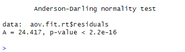
In the Anderson-Darling test for normality on the reaction time data for the normal-hearing group, the null hypothesis is that the residuals are normally distributed. The test result shows a statistic of A = 24.4 and a p-value smaller than 0.05. Since the p-value is smaller than the significance level of 0.05, we reject the null hypothesis. In conclusion, the residuals from the ANOVA using reaction time data as the dependent variable may not be normally distributed.
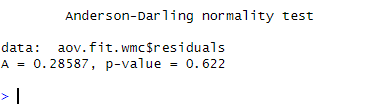
The Anderson-Darling test for normality was conducted on the model’s residuals using working memory capacity as the dependent variable. The results show that the test statistic (A) is 0.29, and the p-value is 0.62. Since the p-value is greater than the significance level of 0.05. In conclusion, we fail to reject the null hypothesis that the residuals are normally distributed. Therefore, we can assume that the residuals are normally distributed.
Report the Anderson-Darling Test: APA 7
We can report the results like this:
The Anderson-Darling test for normality was performed on the reaction time model, and the results showed that the residuals were not normally distributed (A =24.4 , p < .001). The same test was performed on the working memory capacity model, and the results showed that the residuals were normally distributed (A = 0.29, p = .62).
As discussed in another section about interpreting the Shapiro-Wilks test, it is important to keep in mind that we should not rely solely on statistical tests for checking normality assumptions. Diagnostic checks, such as visual inspection of histograms or Q-Q plots, can help confirm the ANOVA results. Furthermore, violations of normality assumptions may not necessarily pose a problem.
In the following section, we will look at another test for normality that we can carry out using R.
Kolmogorov-Smirnov Test for Normality
To carry out the Kolmogorov-Smirnov Test for Normality in R, we can use the ks.test() function from the stats package. This function tests whether a sample comes from a normal distribution by comparing the sample’s cumulative distribution function (CDF) to the CDF of a standard normal distribution.
Here are the code chunks for performing the Kolmogorov-Smirnov Test for Normality in R on the same example data:
Non-Normal Data
Here is an example of the reaction time data:
aov.fit.rt <- aov(RT  ~ Hearing, data = psych_data)

ks.test(aov.fit.rt$residuals, "pnorm", mean = mean(aov.fit.rt$residuals),
        sd = sd(aov.fit.rt$residuals))Code language: PHP (php)
Normal Data
Here is an example of the working memory capacity data:
aov.fit.wmc <- aov(WMC  ~ Hearing, data = psych_data)

ks.test(aov.fit.wmc$residuals, "pnorm", mean = mean(aov.fit.wmc$residuals),
        sd = sd(aov.fit.wmc$residuals))Code language: R (r)
In the two code chunks above, we run an ANOVA using the aov function in R with RT and WMC as dependent variables and ‘Hearing’ as the independent variable. Next, we use the ks.test function to perform a Kolmogorov-Smirnov test on the residuals of each ANOVA. The pnorm argument specifies that the test should be performed against a normal distribution, and the ‘mean’ and ‘sd’ arguments specify the mean and standard deviation of the normal distribution. The KS test compares the sample distribution to the normal distribution and returns a p-value.
Interpreting the Kolmogorov-Smirnov Test
In the code chunk, the Kolmogorov-Smirnov test for normality was conducted on the RT data for participants with normal hearing. The test statistic, D, was 0.24, and the p-value was smaller than 0.05. This indicates that the distribution of RT scores is significantly different from a normal distribution. We get similar results for the hearing-impaired group.
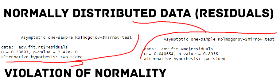
In the third code chunk, the Kolmogorov-Smirnov test for normality was conducted on the WMC data for participants with normal hearing. The test statistic, D, was 0.04, and the p-value was 0.89. This indicates that the distribution of WMC scores is not significantly different from a normal distribution. We get similar results for the hearing-impaired group.
How to Report the Kolmogorov-Smirnov Test: APA 7
We can report the results from the Kolmogorov-Smirnov test for normality like this:
For the one-sample Kolmogorov-Smirnov tests, we found that the distribution of residuals was significantly different from a normal distribution (D = 0.24, p < .001). . For the model including working memory capacity as a dependent varable, the distribution of residuals did not significantly deviate from normality (D = 0.04, p = .89).
Again, violations of normality assumptions may only sometimes be problematic, particularly with large sample sizes or mild deviations from normality. See the previous sections on interpreting the Shapiro-Wilks and Anderson-Darling tests for more information.
Dealing with Non-normal Data
If the residuals are non-normal, we can explore the reasons for the non-normality, such as outliers or skewed distributions, and try to address them if possible.
For ANOVA, violations of normality assumptions are less of a concern when the sample sizes are large (typically over 30). The central limit theorem indicates that the distribution of means of samples taken from a population will approach normality regardless of the original population distribution.
In such cases, the ANOVA results may still be reliable even if the residuals are not normally distributed. However, suppose the sample sizes are small or the deviations from normality are severe. In that case, the ANOVA results may not be trustworthy, and non-parametric tests or data transformation techniques may be more appropriate.
Z-Score Transformation
One approach to handling non-normal data is to transform it to achieve normality. Z-score transformation is one option to standardize the data and can be helpful in some non-normal distributions. However, it is not always appropriate, and other types of transformations, such as log or square root transformations, may be more suitable depending on the data and research question. It is important to remember that the interpretation of the transformed data may be less intuitive, and the results should be carefully evaluated in the context of the research question. Additionally, if the non-normality is severe or cannot be adequately addressed by transformation, it may be necessary to use non-parametric statistical tests instead of traditional parametric tests.
Non-Parametric Tests
Several non-parametric tests, such as the Wilcoxon rank-sum, Kruskal-Wallis, and Mann-Whitney U tests, can be used when data is not normally distributed. These tests do not assume normality and can be more appropriate when dealing with non-normal data. Here are some resources on this blog that may be useful:
Additional Approaches
Testing for normality in R is just one tool for assessing normality. It is also important to examine the residual distribution visually using histograms, density plots, and Q-Q plots. Additionally, it is important to consider the context of the data and the research question being asked. Sometimes, even if the data is not perfectly normal, it may be appropriate to use parametric tests if certain assumptions are met. Another reason is that the deviations from normality are minor. Therefore, it is important to use a combination of statistical tests and visual inspection to make decisions about the normality of the data.
Conclusion: Test for Normality in R
This blog post was about the importance of testing for normality in data science and psychology. We covered various methods to test for normality in R, including the Shapiro-Wilks, Anderson-Darling, and Kolmogorov-Smirnov tests. We also discussed interpreting and reporting these tests according to APA 7 guidelines.
Testing for normality is important in many statistical analyses, as parametric tests assume normality of the residuals. Violations of normality can lead to inaccurate results and conclusions. Therefore, it is essential to use appropriate methods to test for normality and, if necessary, apply appropriate transformations or non-parametric tests.
In addition to the technical aspects, we provided real-world examples of normal and non-normal data in both data science and psychology contexts. We also discussed additional approaches for non-normal data (i.e., when the residuals deviate).
By mastering the methods for testing for normality in R, you will be better equipped to conduct rigorous statistical analyses that produce accurate results and conclusions. We hope this blog post was helpful in your understanding of this crucial topic. Please share this post on social media and cite it in your work.
Resources
Here are other blog posts you may find helpful:
- How to use %in% in R: 8 Example Uses of the Operator
- Sum Across Columns in R – dplyr & base
- How to Calculate Five-Number Summary Statistics in R
- Durbin Watson Test in R: Step-by-Step incl. Interpretation
- R Count the Number of Occurrences in a Column using dplyr
- How to Add a Column to a Dataframe in R with tibble & dplyr
- Mastering SST & SSE in R: A Complete Guide for Analysts
- How to Transpose a Dataframe or Matrix in R with the t() Function