Mastering SST & SSE in R: A Complete Guide for Analysts

Calculating the sum of squared residuals (SSR, also known as the sum of squared errors; SSE) in R can give us insights into the quality of our statistical models. In addition, computing the total sum of squares (SST) is important for understanding the overall variability in the data. Whether you are a Psychology or hearing science researcher, these calculations can give you a robust framework. For example, we can evaluate model performance and draw meaningful conclusions by using them.

In psychology, understanding SSE in R can allow us to evaluate the accuracy of a predictive model. Moreover, it can enable us to determine how well our model fits the observed data. By quantifying the discrepancies between predicted and actual values, we can get information about the effectiveness of our theories and hypotheses. Similarly, in hearing science, we can can calculate SSR in R when analyzing auditory perception and assessing the performance of models predicting listeners’ responses. This evaluation aids in fine-tuning ourmodels and optimizing their predictive capabilities.

SSE/SSR & SST in R — Sum of Squares (Error and Total)

Moreover, the computation of SST in R plays can have an essential role in both fields. By capturing the total variability in the data, SST allows us to differentiate between the inherent variation within the data and the variability accounted for by the model. This information can be used to examine the model’s explanatory power and discerning the significance of the predictors under investigation.

In the next section, the outline of the post will be described, followed by a step-by-step guide on how to calculate SSE/SSR, and SST in R. By following this guide, you will gain a solid understanding of these calculations. Moreover, you will learn how to use them effectively in your research and data analysis.

Outline
Requirements
What are These Different Sum of Squares?

Synthetic Data
Fit a Linear Model in R
How to Calculate SST in R

How to Find the SSR in R
- Calculating the SSR Method 1
- Finding the SSE Method 2.
How to Calculate the SSE, SSR, and SST from an ANOVA in R

Conclusion
Resources

Outline

The post begins by discussing the requirements for calculating the sum of squared errors (SSE), also known as the sum of squared residuals (SSR), and the total sum of squares (SST) in R. We will then be answering the questions of what SSE, SSR, and SST are, providing explanations and highlighting their significance. Next, the post demonstrates how to fit a linear model in R and subsequently guides the readers through calculating SST and SSR/SSE. The post also explains how these calculations can be performed using an ANOVA object. Throughout the content, active examples and code snippets illustrate the concepts. Lastly, the post summarizes the key points covered. Here the emphasis is on the importance of understanding and calculating SSE and SSR/SST in statistical analysis.

Requirements

The requirement for this post is to have a basic understanding of statistical analysis and regression models. Familiarity with R statistical programming language, including the usage of functions like lm(), %in%, and dplyr package, is essential. You should also run the latest version of R (or update R to the latest version). Additionally, a foundational understanding of the concepts (e.g., SSE/SSR, & SST) is necessary. You should, furthermore, be comfortable with data manipulation using dplyr, conditional operations with %in%, and fitting linear regression models using lm(). Prior knowledge of ANOVA (Analysis of Variance) and its use in R would be beneficial. The post assumes readers have a dataset available to perform the calculations.

What are These Different Sum of Squares?

This section will briefly describe the SSE/SSR, and SST.

What is the sum of squared errors (SSE/SSR)?

The sum of squared errors (SSE) is a statistical measure that quantifies the overall discrepancy between observed data and the predictions made by a model. It calculates the sum of the squared differences between the actual values and the corresponding predicted values. SSE is commonly used to evaluate regression or predictive models’ accuracy and goodness of fit. A lower SSE indicates a better fit, meaning the model’s predictions align more closely with the observed data. The sum of Squared Errors is sometimes called the Residuals sum of squares.

What is the total sum of squares (SST)?

The total sum of squares (SST) is a statistical measure representing a dataset’s total variability. It quantifies the sum of the squared differences between each data point and the overall mean of the dataset. SST provides a baseline reference for understanding the total variation in the data before any predictors or models are considered. By comparing the SST with the sum of squared residuals (SSR), one can assess how much of the total variation is accounted for by the model. SST is essential in calculating the coefficient of determination (R-squared) to evaluate the model’s explanatory power.

In the next section, we will generate fake data that we will use to calculate the SSE, SSR, and SST in R.

Synthetic Data

Here we use the dplyr package to generate fake data:

library(dplyr)

# Creating a fake dataset
set.seed(123)  # Set seed for reproducibility

# Variables
group <- rep(c("A", "B", "C"), each = 10)
x <- rnorm(30, 50, 10)
y <- ifelse(group %in% c("A", "B"), x * 2 + rnorm(30, 0, 5), x * 3 + rnorm(30, 0, 5))

# Creating a data frame
data <- data.frame(group, x, y)

# Standardizing the data
data <- data %>%
  mutate(
    x_std = scale(x),
    y_std = scale(y)
  )Code language: R (r)

In the code chunk above, we create a fake dataset with three groups (A, B, and C) and two variables (x and y). The values of x are randomly generated from a normal distribution, and y is calculated based on the groups and x, with added noise. Note the %in% operator in R is used in the ifelse statement to check whether the values in the group variable are either “A” or “B”. Specifically, the expression group %in% c("A", "B") is evaluated for each element in the group variable. Next, we create a dataframe called data and then use mutate from dplyr to create standardized versions of x and y using the scale function. This dataset will be used to calculate SSE, SSR, and SST in the following parts of the blog post. In the next section, we will fit a regression model using the data above.

Fit a Linear Model in R

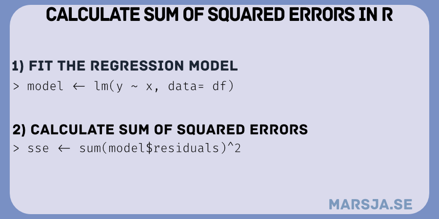
Here is how to fit a linear regression model in R:

model <- lm(y ~ x, data = data)Code language: R (r)

In the code chunk above, we fitted a linear model using the lm() function. Of course, we used the fake data. However, if you use your own data, make sure to replace y with the name of your dependent variable. Furthermore, you need to replace x with the name of your independent variable (and add any more you have). Finally, adjust data to the name of your dataset.

Probit Regression in R: Interpretation & Examples

How to Calculate SST in R

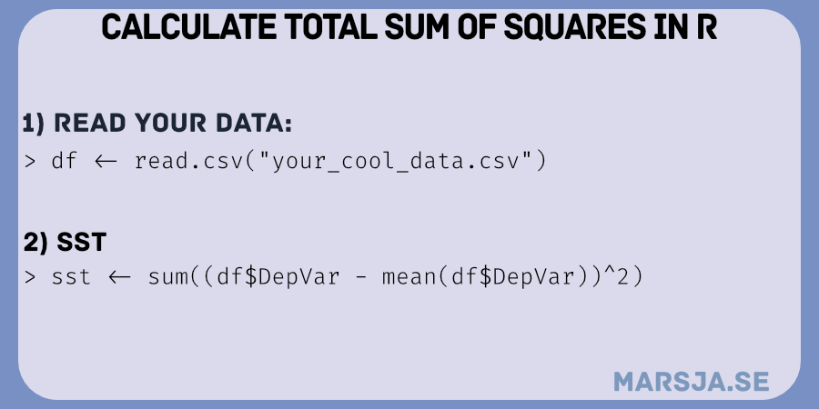
Here is a general code chunk for calculating the total sum of squares in R:

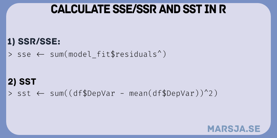
SST <- sum((data$y - mean(data$y))^2)Code language: PHP (php)

In the code chunk above, twe calculate the total sum of squares (SST) using a formula. First, we calculate the mean of the dependent variable y iby using the mean function on data$y. This provides the average value of y across all observations.

Next, we use each individual observation of y in the dataset data and subtract them from the mean value. This subtraction is performed for every observation and creates a vector of deviations from the mean. Next, we use these deviations are squared using the ^2 operator.

Finally, the we use the sum function on the squared deviations, resulting in the sum of all the squared differences between each observation of y and the mean value.

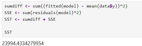
Note that the SST can be calculated in R by summing the sum of squared differences between predicted data points and SSE. In the next section, we will calculate the residual sum of squares in R using the model (e.g., the results from the regression model we previously fitted).

sse in R — residuals sum of squares in R

How to Find the SSR in R

Here are two methods that we can use to calculate the sum of squared errors using R:

Calculating the SSR Method 1

Here is one way to find the SSR in R:

SSR <- sum(residuals(model)^2)Code language: R (r)

In the code chunk above, we calculated the sum of squared residuals in R using a formula. First, we use the residuals function to the model. This function calculates the differences between the dependent variable’s observed values and the model’s corresponding predicted values. These differences are referred to as residuals.

Next, we use the ^2 operator to square each residual, element-wise. Squaring the residuals ensures that positive and negative differences contribute positively to the overall SSR calculation. Finally, the sum function is used to add up all the squared residuals, resulting in the SSR.

Finding the SSE Method 2.

Here is how we can find the sum of squared errors in R:

SSR <- sum((data$y - predict(model))^2)Code language: PHP (php)

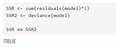
In the code chunk above, we calculate the SSE in R using a formula (the same as SSR). First, we use the predict function on the model. This function generates predicted values of the dependent variable based on the model’s coefficients and the predictor variables in data.

Next, we subtract each observed value of the dependent variable y in datafrom the corresponding predicted value. This subtraction calculates the difference or error between the observed and predicted values for each data point. We then square the errors using the ^2 operator. Finally, the sum function adds up all the squared errors, resulting in the sum of squared errors (SSE).

As seen in the image above, we can also use the deviance function to calculate the SSE.

How to Calculate the SSE, SSR, and SST from an ANOVA in R

To perform the above calculations using an ANOVA object in R, you can utilize the anova() function and a fitted ANOVA model. Here is an example using the built-in dataset mtcars:

# Fitting an ANOVA model
model <- lm(mpg ~ cyl + hp, data = mtcars)
anova_result <- anova(model)

# Extracting SSE from lmobject
SSE <- sum(model$residuals^2)

# Calculating SST
SST <- sum((mtcars$mpg - mean(mtcars$mpg))^2)Code language: R (r)

In the code chunk above, we fit an ANOVA model to explore the relationship between the dependent variable mpg and the independent variables cyl and hp. We utilized the lm() function to perform the linear regression analysis, with mtcars dataset serving as the data source.

Next, we applied the anova() function to the fitted model, resulting in the anova_result object that contains the ANOVA table. Here are the results:

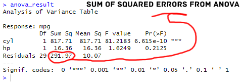
To extract the sum of squared errors (SSE) from the fitted object, we squared the residuals obtained from modelusing the ^2 operator and summed them up using sum(). Just like in the previous examples. Notice that we already have the SSE in the ANOVA table.

Finally, for calculating the total sum of squares (SST), we subtracted each observed value of mpg from the mean of mpg in mtcars, squared the differences, and summed them using sum().

Conclusion

In this post, we have learned how to calculate SSE/SSR and SST in R. We discussed the importance of these measures in statistical analysis and regression modeling. By fitting a linear model in R using the lm() function, we gained hands-on experience in applying regression techniques.

Throughout the post, we learned the step-by-step process of calculating SST/SSR and SSE. We learned how to find the total sum of squares by calculating the squared deviations from the mean, determine the sum of squared residuals by squaring and summing the residuals, and calculate the sum of squared errors by comparing observed and predicted values.

Moreover, we demonstrated the calculations using an ANOVA object, showcasing another approach to obtaining SSE, SSR, and SST. By understanding these calculations, researchers and analysts can better assess model performance and interpret the variation in their data.

I hope this post has provided you with a comprehensive understanding of SSE, SSR, and SST in R. By sharing this post on your favorite social media platforms, you can help others to learn these fundamental concepts. Furthermore, I encourage you to refer back to this post in your work, whether it be research papers, reports, or blog posts, to enhance the accuracy and clarity of your statistical analysis.

Resources

Here are some resources you may find helpful: