How to Create a Word Cloud in R

In this blog post, we will learn how to create a word cloud in R. A word cloud is a captivating way to present text data, highlighting the frequency of words in a visually appealing manner. By creating word clouds in R, we can gain valuable insights from our text data and identify key patterns and trends.

Throughout this tutorial, we will explore various aspects of word clouds in R, from using built-in functions to generating word clouds from CSV files. We will delve into creating word clouds and customizing them to suit our needs. Word clouds can provide valuable information to analyze search results, examine customer feedback, or explore survey textual data.

We will also discover how to remove irrelevant words from word clouds, ensuring that the visualization focuses on the most important insights. Additionally, we will explore the possibility of creating word clouds in the form of bubbles, adding an extra layer of visual appeal to the presentation.

Moreover, we will cover creating a word cloud of search results in R, enabling you to gain meaningful insights from search data. The process is user-friendly and offers powerful analysis capabilities.

This tutorial will equip you with the skills to create compelling word clouds in R, making data analysis and communication an effortless experience. The word cloud package in R will be your ally in this endeavor as we explore its features and functionalities.

Let us dive into word clouds in R and unleash the potential of visualizing textual data. The following section will outline the content of the post in detail.

Outline

The outline of the post is structured to provide a comprehensive guide to creating word clouds in R. To follow this tutorial, basic familiarity with R and data manipulation is helpful. We will use the tm and wordcloud packages for text preprocessing and generation of word cloud.

In the first section, we introduce the prerequisites, which include the packages needed to follow this post.

Next, we present a short step-by-step guide to creating word clouds in R. The guide covers data preparation using the tm package, including converting text to lowercase, removing punctuation, numbers, and stopwords.

Following that, we delve into the syntax of the wordcloud function in R. We explore various arguments like scale, min.freq, rot.per, and colors to customize the word cloud appearance and emphasize specific words or themes.

In the subsequent section, we provide a more detailed step-by-step guide to creating word clouds using data from a CSV file. We will read the data, preprocess it, and generate a word cloud, explaining each code step.

In the customization section, we explore additional options to enhance the word cloud’s visual appeal, such as custom colors and rotated words.

Finally, we conclude the post by demonstrating how to read data from a text file and create a word cloud. This enables us to handle text data from different sources and visualize it effectively. Throughout the post, we use short sentences and provide explanations to facilitate an easy-to-follow learning experience.

Word Clouds

A word cloud is a visual representation of text data, where words are displayed in varying sizes based on their frequency in the given text. It provides an intuitive and engaging way to present large amounts of textual information, allowing patterns and prominent terms to stand out vividly. We can use word clouds for data exploration, sentiment analysis, and content summarization.

We can use word clouds to identify frequently mentioned terms in data exploration quickly. They give us a glimpse into the main themes or topics present in the text. This technique is handy for analyzing survey responses, customer feedback, social media posts, and other forms of unstructured data.

For sentiment analysis, word clouds can reveal prevailing sentiments by visualizing the most common words associated with positive or negative sentiments. Additionally, word clouds can be applied to analyze customer reviews, online discussions, or social media sentiments. As a result, they provide valuable insights for businesses and organizations. By utilizing word clouds in this way, companies can better understand public opinions and make data-driven decisions.

Word clouds condense lengthy text documents into visually striking representations in content summarization, offering a quick overview of the most prominent words and themes. Here they facilitate the rapid grasp of key insights, making it an efficient tool for content summarization and information extraction.

Example

An example of word cloud usage in psychological research is examining responses from open-ended survey questions. Researchers can create word clouds to visualize the most frequently mentioned words or themes in participants’ responses. They help us identify prevalent sentiments, recurring issues, or everyday topics, aiding in data-driven conclusions and qualitative analysis.

word cloud created in R — Word Cloud Psychology Example

Word clouds are versatile tools that enhance data visualization and simplify complex textual information. Their user-friendly nature makes them accessible to various fields, including marketing, social sciences, education, and beyond. Using word clouds, we can extract valuable information, identify trends, and communicate findings effectively.

Prerequisites

Before we delve into creating beautiful word clouds in R, let us ensure you have the necessary prerequisites. Familiarity with basic R programming concepts and data manipulation will benefit this tutorial.

We will use the tm package for text preprocessing and the wordcloud package for creating word clouds. Make sure these packages are installed by using the install.packages() function:

install.packages(c('tm', 'wordcloud'))Code language: R (r)

To ensure that your R environment is up-to-date with the latest features and security enhancements, regularly update both R and RStudio. With these prerequisites, we can explore the exciting world of word cloud creation in R.

A step-by-step guide to creating a word cloud in R:

Install and load necessary packages: Ensure you have the required packages, such as tm, wordcloud, and tm.plugin.webmining, installed and loaded.
Prepare your text data: Load your text data into R, whether from a CSV file, web scraping, or any other source.
Data preprocessing: Perform text preprocessing tasks like converting to lowercase, removing punctuation, and eliminating stop words.
Create a term-document matrix: Transform your text data into a term-document matrix using the tm package.
Generate the word cloud: Use the wordcloud package to create the visualization.
Customize the word cloud: Customize the appearance of the word cloud by adjusting parameters like color, size, and word frequency.
Remove irrelevant words (optional): Remove specific words from the word cloud to focus on key insights.
Save and export (optional): Save the word cloud image as a file or export it to share with others.

Throughout the post, we will detail each step, exploring different techniques and customizations.

The Syntax of the wordcloud Function in R:

The wordcloud() function in R is a powerful tool for creating visually appealing word clouds from text data. Here is a breakdown of its key arguments:

words: A vector of words to be plotted in the word cloud.
freq: A vector of frequencies corresponding to each word in the “words” vector.
scale: A vector of two values indicating the range of font sizes for the words in the word cloud.
min.freq: The minimum frequency threshold for words to be included in the word cloud.
max.words: The maximum number of words to be displayed in the word cloud.
random.order: A logical value indicating whether words should be displayed randomly.
random.color: A logical value indicating whether to use random colors for the words.
rot.per: The proportion of words that should be displayed at a random angle (rotated).
colors: The color(s) to be used for the words in the word cloud.
ordered.colors: A logical value indicating whether the colors should be ordered.
use.r.layout: A logical value indicating whether to use R’s layout engine for word placement.
fixed.asp: A logical value indicating whether to use a fixed aspect ratio for the word cloud.

With these arguments, we can customize the appearance and layout of the word cloud. Experiment with different settings to create visually striking and informative word clouds that effectively visualize the frequency of words in our text data.

Preparing Text Data for Word Cloud in R

Before creating a word cloud in R, we must have our text data ready for analysis. This tutorial will use the read.csv function to load the data from a CSV file. However, we can also acquire text data from web scraping, APIs, or other sources.

Loading Data in R

To load data from a CSV file, follow these steps:

Ensure the CSV file is in the working directory or provide the file path.
Use the read.csv function to read the data into R as a data frame.
Assign the dataframe to a variable for further processing.

Here we read an example dataset into R:

# Load data from a CSV fil
hearing_df <- read.csv("./hearing_data.csv")Code language: R (r)

In the code chunk above, we use the read.csv function in R to read a CSV file named “hearing_data.csv” (or your .csv file). The read.csv function enables us to import the data from the CSV file and store it in the variable hearing_df.

Before running this code, ensure that the “hearing_data.csv” file is present in the working directory of the R session. If the file is in a different location, specify the path accordingly (e.g., “C:/path/to/hearing_data.csv”). The following section will teach us how to prepare the data before making a word cloud in R.

Preparing Data in R

Once the data is loaded, the next step is to prepare it for creating the word cloud. This preparation involves cleaning and preprocessing the text to remove unwanted elements and convert it into a suitable format.

The key preprocessing steps include:

Converting text to lowercase to ensure case-insensitive analysis.
Removing punctuation marks that do not add meaning to the word frequency.
Eliminating common stopwords, such as “the,” “and,” “is,” which are frequently occurring but do not contribute much to analysis.

Here is an example using the data we loaded into R in the previous section:

library(tm)

# Preprocess the text data assuming the text data is stored in the "Statement" column of the dataframe
hearing_clean <- tm_map(hearing_df$Statement, content_transformer(tolower))
hearing_clean <- tm_map(hearing_clean, removePunctuation)
hearing_clean <- tm_map(hearing_clean, removeNumbers)
hearing_clean <- tm_map(hearing_clean, removeWords, stopwords("english"))Code language: R (r)

In the code chunk above, we utilize the tm package to preprocess the text data stored in the Statement column of the dataframe hearing_df. This preprocessing involves converting the text to lowercase using the content_transformer(tolower) function to ensure uniformity in text analysis. Additionally, we remove punctuation from the text data using the removePunctuation function and eliminate numbers using the removeNumbers function.

After these initial steps, we proceed to remove common stopwords (e.g., “the,” “and,” “is”) from the text data using the removeWords function in R, with the argument stopwords("english"). This step helps us focus on the meaningful words in the statements when creating word clouds, providing a more insightful representation of the text data.

By cleaning the text data, we prepare it for further analysis, such as creating word clouds displaying the most frequently occurring words. The preprocessing steps ensure that the word cloud highlights the keywords and concepts related to hearing problems, providing valuable insights into the prevalent issues individuals with hearing loss face.

Importantly, we must perform data preprocessing steps before creating the word cloud in R. These steps include converting to lowercase, removing punctuation, and eliminating stopwords to obtain meaningful and impactful visualizations.

Create a term-document Matrix

After preprocessing the text data, the next step is transforming it into a term-document matrix. Again, we will use the tm package in R. This matrix represents word frequencies in the text data.

Here is how to create the term-document matrix:

Create a Corpus, a collection of text documents from the preprocessed text data.
Use the TermDocumentMatrix function to convert the Corpus into a term-document matrix.
The term-document matrix provides the data needed to create a word cloud, visually displaying word frequencies.

Here is how we can do it on the example data:

# Optional if already loaded
library(tm)

# Create a Corpus from the preprocessed text data 'hearing_clean' using VectorSource()
hearing_corpus <- Corpus(VectorSource(hearing_clean))

# Generate a term-document matrix ('hearing_tdm') from the Corpus to represent word frequencies.
hearing_tdm <- TermDocumentMatrix(hearing_corpus)

# Convert the term-document matrix to a regular matrix ('hearing_matrix') for further analysis.
hearing_matrix <- as.matrix(hearing_tdm)

# Calculate the total word frequencies and sort them in decreasing order.
hearing_words <- sort(rowSums(hearing_matrix), decreasing = TRUE)

# Create a data frame ('hearing_words_df') with the sorted words and their corresponding frequencies.
hearing_words_df <- data.frame(Word = names(hearing_words),
                               Frequency = hearing_words)
Code language: R (r)

In the code chunk above, we use the tm package in R to construct a term-document matrix from the preprocessed text data stored in the variable hearing_clean. If the package is not already loaded, we load it.

The next step involves creating a Corpus using VectorSource(hearing_clean), which converts the preprocessed text data into an appropriate format for further analysis. Subsequently, we apply TermDocumentMatrix() to the Corpus, resulting in the term-document matrix hearing_tdm. By converting hearing_tdm into a regular matrix, hearing_matrix, we prepare the data for calculating word frequencies. Sorting the word frequencies in decreasing order, we obtain the variable hearing_words. To visualize the word cloud, we create the dataframe hearing_words_df, containing the sorted words and their corresponding frequencies. With the term-document matrix ready, we can now generate the word cloud in R and explore the insights it offers from the text data.

Next, utilizing the dataframe hearing_words_df, we create the word cloud, visually representing the most frequent words in the text data. This step allows us to gain valuable insights and identify significant patterns in the text. The subsequent sections will guide us through creating the word cloud and further analyzing the results.

Generating the Word Cloud in R

The final step in creating a word cloud is to use the wordcloud package, which allows us to create an eye-catching visual representation of word frequencies. This visualization will help us understand the prominence of different words in the text data.

To generate the word cloud, follow these steps:
Load the wordcloud package in R if you still need to.

Create the word cloud using the wordcloud() function, passing the term-document matrix (e.g., hearing_tdm) as input. The wordcloud function automatically takes care of the word frequencies.

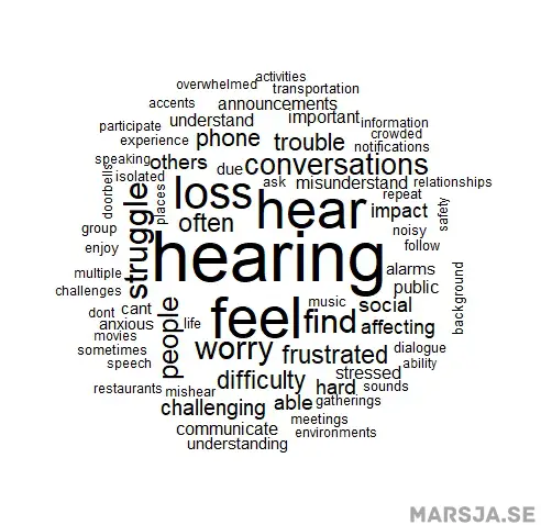
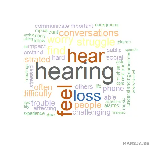
Here is how we can create a word cloud using the wordcloud function in R:

# Load the 'wordcloud' package
library(wordcloud)

# Create the word cloud visualization from the term-document matrix 'hearing_tdm'
wordcloud(words = hearing_words_df$Word, freq = hearing_words_df$Frequency,
          random.order = FALSE)Code language: PHP (php)

In the code chunk above, we load the wordcloud package, which provides functions for creating word cloud visualizations in R. After loading the package, we generate the word cloud using the term-document matrix ‘hearing_tdm’ we previously created. The ‘wordcloud’ function is responsible for creating the visualization, and we provide the necessary data as arguments. Specifically, we use hearing_words_df$Word to supply the words displayed in the word cloud and hearing_words_df$Frequency to provide the corresponding word frequencies. By setting random.order to FALSE, we ensure that the words are displayed in a deterministic order based on their frequencies, making the visualization more interpretable and informative. The resulting word cloud visually represents the most frequent words in the text data, offering insights into the recurring themes or issues related to hearing problems. The size of each word in the word cloud corresponds to its frequency, making the more frequently occurring words stand out prominently. Here is the result:

word cloud in R — Word Cloud Created in R

Here are a couple of more data visualization tutorials:

In the next section, we will learn how to use some of the arguments of the wordcloud to customize the word cloud.

Customizing the Word Cloud in R

Once we have generated the word cloud, we can further enhance its appearance and tailor it to our specific needs by customizing various parameters of the wordcloud function in R. This section will explore some key arguments allowing us to customize the word cloud visualization.

Color of the Word Cloud

One method to change the color of the word cloud in R is to use the brewer.pal function. By specifying the number of colors and the desired palette name, such as “Accent,” we can easily customize the color scheme of the word cloud. Here is an example:

wordcloud(words = hearing_words_df$Word, freq = hearing_words_df$Frequency,
          random.order = FALSE, colors = brewer.pal(8, "Accent"))
Code language: R (r)

In this code chunk, we create the word cloud using the wordcloud function. Moreover, we set the colors argument to brewer.pal(8, 'Accent'). This means the word cloud will use the “Accent” color palette from the brewer.pal function with 8 different colors.

The brewer.pal function provides various color palettes, each designed to make the visualization more visually appealing and easier to read. The first argument in the function specifies the number of colors we want in the palette (e.g., 8 colors). Additionally, the second argument is the palette’s name (e.g., “Accent”). You can experiment with different palettes and color combinations to find the one that best suits your data and enhances the overall appearance of the word cloud.

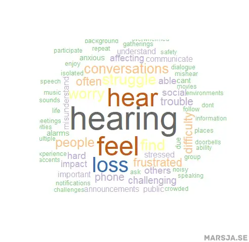
Using brewer.pal to customize the colors of your word cloud can significantly improve the presentation of your text data, making it more engaging and informative. Feel free to try out different palettes and explore how each one affects the visual representation of your word cloud.

Font Size Control

The scale argument in the wordcloud function allows us to control the font size of words displayed in the word cloud. Adjusting the scale allows us to emphasize certain words based on their importance or frequency visually. A larger scale value will increase the font size, making those words more prominent, while a smaller scale value will reduce the font size, making less frequent words appear smaller.

We can adjust the font size scale to emphasize the most common words more. Here is an example of how to do it:

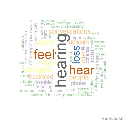
# Create the word cloud visualization from the term-document matrix 'hearing_tdm'
wordcloud(words = hearing_words_df$Word, freq = hearing_words_df$Frequency,
          random.order = FALSE, colors = brewer.pal(8, "Accent"), scale = c(5, 0.5))
Code language: R (r)

We adjusted the scale argument to c(5, 0.5) in the code chunk above. This choice makes the largest words five times bigger than the smallest ones. Doing this makes the most frequent words stand out more prominently in the word cloud. Here is the result:

Change the Frequency of Included Words

Now, suppose we want to set a minimum frequency threshold of 5. Words that occur less than five times will be excluded from the word cloud. Here is how to do it:

# Create the word cloud visualization with the min.freq argument
wordcloud(words = hearing_words_df$Word, freq = hearing_words_df$Frequency,
          random.order = FALSE, colors = brewer.pal(8, "Accent"),
          min.freq = min_frequency_threshold)Code language: PHP (php)

In the code chunk above, we utilized the min.freq argument and set it to 5 when creating the word cloud using R with the wordcloud package. By doing so, we ensured that only words occurring five or more times in the hearing_words_df dataframe were included in the word cloud. This approach allowed us to emphasize the most relevant and frequently occurring words, resulting in a more meaningful and insightful word cloud representation. For further customization, you can easily adjust the min.freq value based on your specific analysis needs, controlling which words appear in the word cloud according to their frequency.

Change the Number of Rotated Words

We can also change how many words that are displayed vertically:

# Create the word cloud visualization with rotated words
wordcloud(words = hearing_words_df$Word, freq = hearing_words_df$Frequency,
          random.order = FALSE, colors = brewer.pal(8, "Accent"),
          rot.per = 0.2)Code language: R (r)

In the code chunk above, we introduced the rot.per argument to create a dynamic word cloud with rotated words. By setting the rot.per value, we can determine the proportion of words that will be rotated by 90 degrees. This addition adds an engaging visual element to the word cloud representation. Adjusting the rot.per parameter allows for a customized and visually appealing word cloud. Consequently, it makes the overall visualization more interesting and captivating.

Save the Word Cloud Created in R

To save a word cloud, we can use the png() or jpeg() functions to create a bitmap image file and then use the dev.off() function to close the device and save the file. Here is an example:

# Save the word cloud as a PNG file
png("word_cloud.png", width = 800, height = 600) # Set the desired width and height
wordcloud(words = hearing_words_df$Word, freq = hearing_words_df$Frequency,
          random.order = FALSE, colors = "grey")
dev.off() # Close the PNG device

# Save the word cloud as a JPEG file
jpeg("word_cloud.jpg", width = 800, height = 600, quality = 90) # Set the desired width, height, and image quality
wordcloud(words = hearing_words_df$Word, freq = hearing_words_df$Frequency,
          random.order = FALSE, colors = "grey")
dev.off() # Close the JPEG deviceCode language: PHP (php)

In the code chunk above, we use the png() function to create a PNG file called “word_cloud.png” with a width of 800 pixels and a height of 600 pixels. Then, we created the word cloud using the wordcloud() function with our data and desired parameters. After creating the word cloud, we use dev.off() to close the PNG device and save the file.

Similarly, we can use the jpeg() function to create a JPEG file with the desired width, height, and image quality and then save the word cloud using the same process.

Make sure to adjust the file names (“word_cloud.png” and “word_cloud.jpg”) and other parameters (width, height, and quality) as per your requirements. Before concluding the post, we will look at reading data from a text file (.txt) and creating a word cloud in R.

Making Word Clouds in R from Text Files

In the previous sections, we learned how to create word clouds in R using data stored in dataframes and how to customize them using various arguments. However, in real-world scenarios, our text data may not always be available in .csv files; it could also be stored in .txt files. This section will explore making word clouds in R using text files.

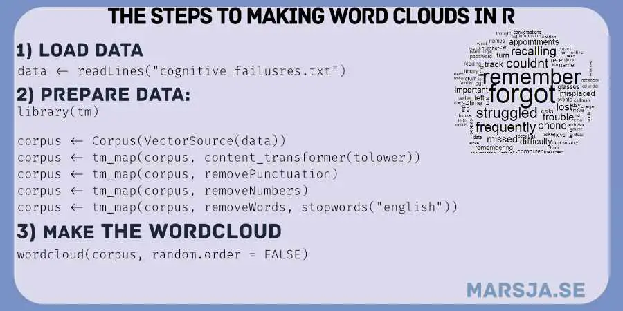
# Step 1: Read data from a text file
cognitive_data <- readLines("cognitive_failures.txt")

# Step 2: Prepare data
library(tm)

cognitive_corpus <- Corpus(VectorSource(cognitive_data))
cognitive_clean <- tm_map(cognitive_corpus, content_transformer(tolower))
cognitive_clean <- tm_map(cognitive_clean, removePunctuation)
cognitive_clean <- tm_map(cognitive_clean, removeNumbers)
cognitive_clean <- tm_map(cognitive_clean, removeWords, stopwords("english"))

cognitive_tdm <- TermDocumentMatrix(cognitive_clean)
cognitive_matrix <- as.matrix(cognitive_tdm)
cognitive_words <- sort(rowSums(cognitive_matrix), decreasing = TRUE)
cognitive_words_df <- data.frame(Word = names(cognitive_words), Frequency = cognitive_words)

# Step 3: Create Word Cloud
library(wordcloud)

wordcloud(words = cognitive_words_df$Word, freq = cognitive_words_df$Frequency, scale = c(5, 0.5),
          random.order = FALSE, colors = brewer.pal(8, "Accent"))Code language: PHP (php)

In the code chunk above, we demonstrate how to create a word cloud in R using data from a text file. We start by reading the text data from the “cognitive_failures.txt” file and then proceed with data preparation, where we clean the text by converting it to lowercase, removing punctuation, numbers, and common stopwords. Next, we create a term-document matrix representing word frequencies in the text data. Finally, with the help of the wordcloud package, we generate a visually appealing word cloud that highlights the most frequently mentioned words in the text file. This process allows us to visualize and analyze the prevalent themes or sentiments in the text data.

Conclusion

In conclusion, this post has provided a comprehensive guide to creating captivating word clouds in R. We explored the step-by-step process, starting from data preparation with the tm package, removing punctuation, numbers, and stopwords to focus on meaningful words. By utilizing the wordcloud package, we visualized word frequencies in a visually appealing manner.

Throughout the post, we learned how to customize word clouds using various arguments like scale, min.freq, and rot.per, enabling us to emphasize specific words and add visual interest. The flexibility of R and the power of the tm and wordcloud packages allow us to handle text data efficiently and creatively.

It is essential to remember that all example data in this post is fictional and not real. These examples demonstrate the concepts and methods, offering aspiring data analysts and researchers a learning opportunity.

Please share this post with your, e.g. colleagues to help them unlock the potential of word clouds in their data analysis. Let us share the knowledge and continue the journey of learning and exploration in the vast world of data analysis and visualization! Comment below if you have any questions or suggestions, and remember to spread the word about this post!

R Tutorials

Here are some other posts and tutorials you may find helpful: