Binning in R: Create Bins of Continuous Variables

Binning in R is a fundamental data preprocessing technique for data analysis and visualization. With binning, we group continuous data into discrete intervals, facilitating a better understanding of patterns and trends. In this comprehensive tutorial, we will practice binning in R. Moreover, we will explore its applications and benefits in various domains.

Binning allows us to simplify complex datasets, making interpreting and drawing meaningful insights easier. By dividing data into bins, we can deal with discrete categories, reduce noise, and highlight important features. This technique is handy when dealing with large datasets, as it aids in managing data efficiently and extracting relevant information.

This tutorial will showcase practical examples and real-world use cases, covering diverse fields like finance, healthcare, and social sciences. You will learn how to implement binning in R using different methods and packages. For example, we will use the cut() function and the dplyr package, all while describing the rationale behind each step.

Additionally, we will discuss the importance of selecting appropriate bin sizes, avoiding common pitfalls, and interpreting the results accurately. By the end of this tutorial, you should grasp how to do binning in R. Hopefully; this will empower you to handle data effectively and derive valuable insights for data-driven decision-making. In the following section, you will find a detailed outline of the post.

Outline
Prerequisites
Syntax of the cut() Function
Syntax of the ntile() Function
Synthetic data
Binning in R with the cut() Function
Binning in R with dplyr, mutate() & cut()
Binning in R with dplyr & mutate()
How to Create Bins in R that are Numeric
How to Calculate Averages Based on a Binning Variable in R
Visualizing Binned Data in R
Conclusion
R Resources

Outline

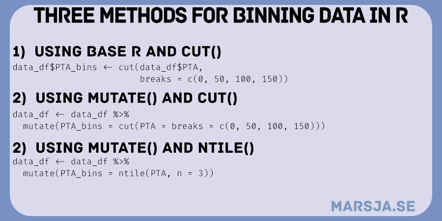
The outline of this post is to provide a comprehensive guide to data binning in R, focusing on two essential functions: cut() and ntile(). We’ll start by exploring the syntax of the cut() function, and learning how to create bins from continuous variables step-by-step. Then, we will look at the ntile() function, which allows us to create numeric bins with equal frequencies for efficient analysis.

To ensure practical application, we will generate synthetic data that simulates two groups’ reaction times and perform binning using various techniques. By combining cut() with dplyr and mutate(), we will demonstrate how to create bins effectively.

Calculating averages based on binning variables is another crucial aspect of data analysis. We will go through the process using dplyr, illustrating how to group data by bins and obtain meaningful averages.

Data visualization plays a significant role in gaining insights; this post will cover it. We will utilize the versatile ggplot2 package to create visually appealing bar plots that showcase distribution across bins.

By the end of this post, you should have a strong understanding of data binning techniques in R, enabling you to apply them in your data analyses. With clear explanations and hands-on examples, this blog post promises to be a valuable resource for beginners and experienced R users. Let us embark on this exciting data binning and analysis journey in R!

Prerequisites

Before we dive into the fascinating world of data binning in R, ensuring you have a solid foundation for this journey is essential. First, basic R programming knowledge is crucial, including understanding data structures, data types, and fundamental syntax. Familiarity with data manipulation techniques, such as filtering, transforming, and summarizing data, will also be beneficial as we explore various binning techniques.

While not mandatory, RStudio provides an excellent integrated development environment (IDE) that enhances the R programming experience. Its features, such as syntax highlighting, code execution, and data visualization, make it a popular choice among R users, streamlining your workflow.

For the data binning techniques we will explore, you must install the dplyr package (if you want to use ntile() and mutate()). dplyr is a powerful and versatile tool for data manipulation tasks. It offers many functionalities, allowing you to easily rename columns, remove duplicates, add new columns, calculate descriptive statistics, and filter data based on specific conditions. For example, with dplyr, you can effortlessly perform operations like renaming columns in R, removing columns, adding new columns, removing duplicates, and counting the number of occurrences in a column.

Additionally, we will visualize our binned data using the versatile ggplot2 package, renowned for its flexibility and ability to create stunning visualizations.

You can use the install to ensure you have the necessary packages installed.packages() function in R:

install.packages(c("dplyr", "ggplot2"))Code language: R (r)

It is also recommended to keep your R version up-to-date to benefit from the latest features, bug fixes, and security enhancements. You can easily update R by downloading a new version or using the updateR() function.

Syntax of the cut() Function

We can use the cut() function to create bins in R. Next, we provide the data to be binned in the x argument. Moreover, we set the breaks argument to specify the breakpoints for the bins. The labels argument allows custom labels for the resulting bins.

We can use the include.lowest argument to include the lowest value in the first bin. Moreover, we use the right to determine whether the intervals should be right-closed or left-closed.

Additionally, we can control the number of decimal places in the labels using the dig.lab argument. If we want the output as an ordered factor, we can use the ordered_result argument.

The … allows additional arguments to be passed to the labels argument. Overall, the cut() function offers flexibility in creating bins from the provided data, making it a powerful tool for data binning in R. Here is a simple example:

Syntax of the ntile() Function

To create bins in R using the ntile() function from dplyr, we utilize the x argument to specify the data for binning. In this context, x is typically the row numbers. However, it can also be any numeric variable representing the data to be divided into bins.

We set the n argument to determine the number of bins we want to create. By choosing the desired value for n, we effectively divide the data into that many equally-sized groups or bins.

The ntile() function then calculates the row numbers’ percentiles and assigns each row to its corresponding bin based on the specified n. Here is a simple example:

Synthetic data

Here is a synthetic dataset tailored for practicing binning in R:

# Load the dplyr package for data manipulation
library(dplyr)

# Set the seed for reproducibility
set.seed(123)

# Generate reaction times (RTs) for Group 1 and Group 2 using rnorm()
group1_rts <- rnorm(100, mean = 500, sd = 100)
group2_rts <- rnorm(120, mean = 550, sd = 120)

# Create a grouping variable "group" using rep()
group <- c(rep("Group 1", 100), rep("Group 2", 120))

# Create a condition variable "condition" using %in% in R
condition <- ifelse(group %in% "Group 1", "Condition A", "Condition B")

# Create an accuracy variable for the groups using sample()
accuracy <- sample(0:1, size = length(group), 
                   replace = TRUE, prob = c(0.4, 0.6))

# Combine the data into a dataframe "rt_df" using data.frame()
rt_df <- data.frame(RT = c(group1_rts, group2_rts), 
                 Group = group, Condition = condition,
                 Accuracy = accuracy)

# Examine the structure and content of the synthetic dataset using head()
head(rt_df)Code language: PHP (php)

In the code chunk above, we use the dplyr package to manipulate and analyze the data in R. By setting the seed to 123 using set.seed(123), we ensure the reproducibility of the random numbers generated in subsequent operations.

We generated synthetic reaction times (RTs) for “Group 1” (100 samples) with a mean of 500 and a standard deviation of 100. Similarly, we generated RTs for “Group 2” (120 samples) with a mean of 550 and a standard deviation of 120 using the rnorm() function.

To create a grouping variable named group, we used the rep() function to repeat the labels “Group 1” and “Group 2” corresponding to the number of RTs in each group.

We used %in% in R to create a “condition” variable. If the group is “Group 1”, it is assigned “Condition A”; otherwise, it is assigned “Condition B”. Here are some tutorials on other helpful operators:

To simulate accuracy values, we utilized the sample() function to randomly select 0s and 1s with probabilities 0.4 and 0.6, respectively, based on the length of each group’s RTs.

Combining all these variables, we created a dataframe rt_df with four columns: RT for reaction times, Group indicating the group information, Condition denoting the condition information, and Accuracy reflecting the accuracy values.

Lastly, using the head() function, we displayed the first six rows of the synthetic dataset to get an overview of its structure and content. Here are the six rows:

In the following section, we will learn how to create bins in R using the cut() function.

Binning in R with the cut() Function

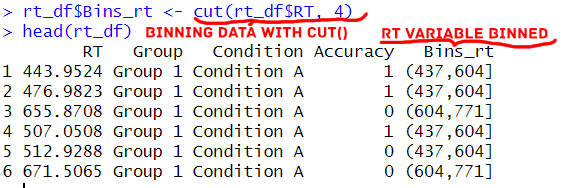
Let us practice binning in R using the synthetic dataset we created. We will employ the cut() function to group the reaction times (RTs) into discrete intervals, allowing us to analyze the data more meaningfully.

# Binning the Reaction Times using the cut() function
df$RT_Bins <- cut(df$RT, breaks = c(400, 500, 600, 700), labels = c("Low", "Medium", "High"))

# Exploring the Binned Data
summary(df$RT_Bins)Code language: PHP (php)

In the code above, we applied the cut() function to bin the reaction times (RTs) in the df dataframe. We divided the RTs into three intervals defined by the breaks argument. We used the breaks 400 to 500, 500 to 600, and 600 to 700. The corresponding labels “Low,” “Medium,” and “High” were assigned to each bin using the labels argument.

To understand the distribution of binned RTs, we used the summary() function to display the summary statistics. Consequently, this revealed the count of RTs in each bin.

By binning the reaction times, we can now observe and compare the distribution of RTs in different intervals. This process provides insights into how the data is distributed across the “Low,” “Medium,” and “High” bins within each condition. In the following section, we will make bins with the mutate() function from dplyr together with the cut() function.

Binning in R with dplyr, mutate() & cut()

We can also use dplyr and mutate() together with the cut() function for binning:

# Binning in R with the cut() function using mutate() from dplyr
library(dplyr)

# Binning the Reaction Times using the cut() function within mutate()
df <- df %>%
  mutate(RT_Bins = cut(RT, breaks = c(400, 500, 600, 700), 
                       labels = c("Low", "Medium", "High"), 
                       include.lowest = TRUE))Code language: PHP (php)

We use cut() within mutate() in the code chunk above. We create a new column called RT_Bins in the df dataframe to store the binned values.

Again, we binned the RT values into three intervals. We defined the intervals using the breaks argument: 400 to 500, 500 to 600, and 600 to 700. Finally, we assigned corresponding labels “Low,” “Medium,” and “High” to each bin using the labels argument.

We set include.lowest = TRUE, to ensure that the lowest interval value (400) is included in the first bin (“Low”), and any RT values falling outside these intervals will be assigned to NA.

cut () within mutate() streamlines the binning process, enabling us to efficiently add the binned values as a new column to the dataframe.

Binning in R with dplyr & mutate()

In this section, we will continue practicing binning in R using the synthetic dataset. Here we will use the mutate() function from the dplyr package to group the reaction times (RTs) into discrete intervals.

library(dplyr)

# Binning the Reaction Times using the mutate() function from dplyr
df <- df %>%
  mutate(RT_Bins = case_when(
    RT >= 400 & RT < 500 ~ "Low",
    RT >= 500 & RT < 600 ~ "Medium",
    RT >= 600 & RT <= 700 ~ "High",
    TRUE ~ NA_character_
  ))
Code language: PHP (php)

In the code chunk above, we used the mutate() function and the case_when() function. We used these functions to create a new column, RT_Bins. Specifically, we defined the binning logic using conditional statements:

RT values between 400 and 500 are labeled as “Low”.
RT values between 500 and 600 are labeled as “Medium”.
RT values between 600 and 700 are labeled as “High”.

Any RT values falling outside these intervals are marked as NA (Not Available) using the TRUE ~ NA_character_ argument.

This approach provides flexibility in specifying custom bin ranges and labels based on your data’s characteristics. The mutate() function allows us to create the new column directly within the dataframe. This makes the binning process more efficient and convenient.

How to Create Bins in R that are Numeric

For creating a set number of bins in R, the ntile() function is ideal. It divides the data into equally sized groups, making it suitable for our needs. Here is how to create numeric bins in R using ntile() within mutate() from dplyr.

# Binning in R with ntile() function using mutate() from dplyr
library(dplyr)

# Specify the number of bins
num_bins <- 3

# Binning the Reaction Times using ntile() function within mutate()
df <- df %>%
  mutate(RT_Bins = ntile(RT, n = num_bins))
Code language: R (r)

In the code above, we use the ntile() function within mutate() to create a new column named RT_Bins in the df dataframe. We specify n = num_bins to create three equally sized bins (num_bins = 3) for the RT values.

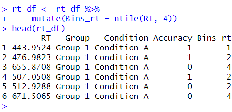
The data is divided into three bins using the ntile() function. Consequently, each contains approximately one-third of the data points. The values in the RT_Bins column will range from 1 to 3, representing the bin numbers to which each RT value belongs.

This approach is beneficial when we want to divide the data into a specific number of numeric bins. Especially when we do not want to define the bin ranges explicitly. In this case, it offers a convenient way to group data into roughly equal-sized intervals. Therefore, ntile() provide an alternative to the cut() function when numeric binning is preferred.

How to Calculate Averages Based on a Binning Variable in R

To calculate averages based on a binning variable in R, we can use the dplyr package. First, we group the data by the binning variable and then calculate the mean for each group. Here is how to calculate averages based on a binning variable in R:

# Load the dplyr package for data manipulation
library(dplyr)

# Group by the binning variable (RT_Bins) and calculate the average for the "RT" variable
averages_df <- rt_df %>%
  group_by(RT_Bins) %>%
  summarize(Average_RT = mean(RT))


# View the resulting dataframe with the averages
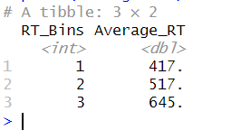
print(averages_df)Code language: R (r)

In the code chunk above, we use group_by() to group the data by the RT_Bins variable. Moreover, we use summarize() to calculate each group’s mean of the Value variable. The result is a new dataframe averages_df containing each bin’s average values. Here is the result:

Visualizing Binned Data in R

If we want to visualize the data binned in R, we can use the ggplot2 package. Here is an example of how to create a bar plot to visualize the binned data:

# Binning in R with ntile() function using mutate() from dplyr
library(dplyr)
# Load the ggplot2 package for data visualization
library(ggplot2)

# Specify the number of bins
num_bins <- 3

# Binning the Reaction Times using cut_number() function within mutate()
rt_df  <- rt_df  %>%
  mutate(RT_Bins = ntile(RT, n = num_bins))

# Create a bar plot to visualize binned data
ggplot(rt_df, aes(x = RT_Bins, fill = Group)) +
  geom_bar(position = "dodge") +
  labs(x = "Binned Reaction Times", y = "Frequency", title = "Binned Data Visualization") +
  theme_bw() +
  theme(panel.grid = element_blank()) Code language: PHP (php)

In the code above, we first used the ntile() function from dplyr to bin the RT data into three bins, as specified by the num_bins variable.

The resulting dataframe rt_df contains the RT_Bins column with bin numbers. We then used ggplot2 to create a bar plot. In the plot, the x-axis represents the binned reaction times (RT_Bins), and the fill color distinguishes the different groups using the “Group” variable. The geom_bar() function creates the bars, and position = "dodge" ensures they are placed side by side.

To improve the plot’s appearance, we used theme_bw() to set a clean and minimalistic theme and theme(panel.grid = element_blank()) removed the background grid lines. Here is the resulting plot:

This visualization allows us to observe the distribution of reaction times across the bins and compare the frequencies of each bin for different groups. This visual representation allows us to gain valuable insights from our binned data and effectively communicate our findings. Here are some other ggplot2 tutorials you may find handy:

Conclusion

In this post, we have explored the syntax and functionality of the cut() function and the ntile() function in R for creating bins and performing binning operations on a continuous variable.

Throughout the post, we utilized synthetic data to demonstrate applying these functions effectively. With the cut() function, we learned how to create bins based on specific breakpoints and assign labels to each bin. This allowed us to group the data into meaningful intervals and analyze patterns within the dataset.

Next, we learned using cut() with mutate() from the dplyr package. By doing so, we seamlessly incorporated the binning process into our data manipulation pipeline, enabling efficient transformations and analyses.

We also explored the ntile() function from dplyr, which allowed us to create numeric bins by specifying the desired number of groups. This method provided a useful alternative for binning data when a specific number of bins was required.

Moreover, we investigated how to calculate averages based on the binning variable. Grouping the data by the bins, we employed the group_by() and summarize() functions from dplyr to obtain the mean values for each bin, gaining further insights into our data’s distribution.

Lastly, we ventured into visualizing binned data using the ggplot2 package. By creating visually appealing plots, we enhanced our understanding of the distribution patterns within the bins.

Now that you have a comprehensive toolkit for binning in R, you can confidently embark on data-binning projects, unravel hidden patterns, and draw meaningful conclusions from your datasets. We encourage you to share this post on social media and tell others about the valuable insights gained through binning. Additionally, I would love to hear your thoughts and experiences with data binning in R. Feel free to comment below and join the conversation.

R Resources

Here are some tutorials you may find helpful: