Coefficient of Variation in Python with Pandas & NumPy

In this tutorial blog post, we will explore how to calculate the Coefficient of Variation in Python using Pandas and NumPy. The Coefficient of Variation is a valuable measure of relative variability that expresses the standard deviation as a percentage of the mean. By understanding the CV, you can gain insights into data spread and stability, enabling you to make informed decisions in your data analysis.

First, we will introduce the formula, interpretation, and significance of the Coefficient of Variation. Then, we will dive into its application using a real-world example from cognitive hearing science, showcasing its practical usage.

Throughout this post, we will leverage the power of Python libraries, particularly Pandas and NumPy, to efficiently calculate the Coefficient of Variation.

By the end of this tutorial, you will clearly understand how to compute the Coefficient of Variation in Python. As a result, you can explore data variability and draw meaningful conclusions from your data. To upload your data, you can use the coefficient of variation calculator.

Outline
Prerequisites
Coefficient of Variation
- Interpretation
Example from Cognitive Hearing Science
Synthetic Data
Calculate the Coefficient of Variation using Python & Pandas
Coefficient of Variation by Group in Python
Calculate the Coefficient of Variation for All Numeric Variables
Calculate the Coefficient of Variation for a Python List
Conclusion
References
Resources

Outline

The outline of this post revolves around the concept of the Coefficient of Variation (CV), a statistical measure used to quantify the relative variability of a dataset. In the first section, we will learn a bit about the CV and how to interpret it.

Next, we will generate synthetic data using Python and Pandas to dig deeper into the concept. Synthetic datasets for both “normal hearing” and “hearing impaired” groups will be created, incorporating SRT values and age data. This step facilitates understanding the CV in a practical context.

Next, we will demonstrate calculating the Coefficient of Variation using Python and Pandas. We will do this for datasets with multiple numeric variables. Using the groupby() and agg() functions enable efficient computation of the CV for each variable within the dataset. Specifically, it enhances data summarization and comparison among different groups.

Additionally, we will show how to calculate the Coefficient of Variation for a Python list using NumPy, providing a straightforward method for individual data points.

Prerequisites

To follow this tutorial, you will need some basic knowledge of Python. Additionally, you should have NumPy and Pandas installed in your Python environment. If you still need to install these libraries, you can use pip, the Python package manager, to install them easily.

To install Python packages, such as NumPy and Pandas, open your terminal or command prompt and use the following commands:

pip install numpy pandas
Code language: Bash (bash)

If pip tells you that there is a newer version of pip available, you can upgrade pip itself:

pip install --upgrade pip
Code language: Bash (bash)

Sometimes, you might need to install a specific version of NumPy or Pandas. You can do this by specifying the version number in the pip install command.

Once you have the needed Python packages installed, you are all set to calculate the Coefficient of Variation in Python.

Coefficient of Variation

The Coefficient of Variation (CV) is a powerful statistical measure that quantifies the relative variability of a dataset. We use it to understand the dispersion of values concerning their average. The formula is simple: divide the standard deviation by the mean and multiply by 100. This normalization allows standardized comparisons across different datasets, disregarding their scales or units.

Formula: CV = (σ / μ) * 100

The CV provides valuable insights when comparing datasets with different means. It considers the proportion of variation relative to the average value. A higher CV suggests greater relative variability, indicating a wider spread of data points around the mean. Conversely, a lower CV implies greater consistency and less dispersion among the values.

Interpretation

Interpreting the CV depends on the context of the data. In clinical psychology, a higher CV might indicate more significant variability in test scores or patient responses, suggesting diverse outcomes. On the other hand, a lower CV suggests greater consistency and reliability of measurements or experimental results.

Using the CV, we can gain valuable insights into the relative variability of our data, which informs decision-making and guides further analysis. It helps identify datasets with high dispersion or wide fluctuations, prompting us to investigate the contributing factors.

In summary, the CV is a powerful tool for measuring and comparing the relative variability of datasets. Its formula normalizes the standard deviation by the mean, facilitating standardized comparisons across different datasets. Understanding the CV enables us to grasp the spread and stability of our data. Moreover, it provides valuable insights that enhance decision-making and deepen our understanding of data patterns.

Example from Cognitive Hearing Science

In Cognitive Hearing Science, the coefficient of variation (CV) is significant in various research applications. Let us consider a study investigating the relationship between working memory performance and hearing impairments in speech recognition in noise, measured by speech reception thresholds (SRTs). SRT is a crucial metric that reflects an individual’s ability to recognize speech in noisy environments. Therefore, it is particularly relevant for those with hearing difficulties.

Suppose we compare the SRTs of individuals with normal hearing (Group A) and individuals with hearing impairments (Group B). In this example, we aim to determine which group shows greater variability in their SRTs. By calculating the CV for each group, we can assess the relative variability of their SRTs compared to their respective means.

If Group A exhibits a higher CV than Group B, it suggests that the SRTs within Group A are more widely dispersed relative to their mean. This could indicate greater inconsistency or fluctuations in speech recognition performance within Group A, despite having normal hearing. On the other hand, if Group B demonstrates a lower CV, it suggests more consistency in their SRTs, despite hearing impairments.

By utilizing the coefficient of variation in this context, we gain insights into the relative variability of SRTs between the two groups. This information can contribute to a better understanding of the relationship between working memory performance and speech recognition abilities in individuals with hearing impairments, potentially revealing important connections and individual differences.

In conclusion, the coefficient of variation serves as a valuable tool in Cognitive Hearing Science to quantify and compare the relative variability of data. It allows researchers to explore patterns, identify differences, and interpret the spread of speech recognition thresholds concerning the mean. Finally, it can provide crucial insights into the intricate interplay between working memory, hearing impairments, and speech perception abilities in noisy environments.

Synthetic Data

Here we generate synthetic data to practice calculating the coefficient of variation in Python:

import pandas as pd
import numpy as np

# Parameters for a "normal hearing" group
normal_mean_srt = -8.08
normal_std_srt = 0.44
normal_group_size = 100

# Parameters for a "hearing impaired" group
impaired_mean_srt = -6.25
impaired_std_srt = 1.6
impaired_group_size = 100

# Generate synthetic data for the normal hearing group
np.random.seed(42)  # For reproducibility
normal_srt_data = np.random.normal(loc=normal_mean_srt, 
                                   scale=normal_std_srt, size=normal_group_size)
# Age
age_n = np.random.normal(loc=62, scale=7.3, size=normal_group_size)

# Generate synthetic data for the hearing impaired group
impaired_srt_data = np.random.normal(loc=impaired_mean_srt, 
                                     scale=impaired_std_srt, size=impaired_group_size)
# Age
age_i = np.random.normal(loc=63, scale=7.1, size=impaired_group_size)

# Create Grouping Variable
groups = ['Normal']*len(normal_srt_data) + ['Impaired']*len(impaired_srt_data)

# Concatenate the NumPy arrays
srt_data = np.concatenate((normal_srt_data, impaired_srt_data))
age = np.concatenate((age_n, age_i))

# Create DataFrame
s_data = pd.DataFrame({'SRT': srt_data, 'Group':groups, 'Age':age})
Code language: Python (python)

In the code chunk above, we used Pandas and NumPy libraries to generate synthetic data for two groups, “normal hearing” and “hearing impaired,” for speech reception thresholds (SRT) as well as age data.

We began by setting the parameters for each group, including the mean and standard deviation of their SRTs and ages and the number of samples in each group. These parameters defined the characteristics of the synthetic data we created.

Next, we used NumPy’s random number generator to generate synthetic data for the “normal hearing” group for both SRT and age. We set a seed value of 42 using np.random.seed(42) to ensure reproducibility. To generate data, we used the np.random.normal() function. For SRT, we created an array (normal_srt_data) of 100 values sampled from a normal distribution with a mean (loc) of -8.08 and a standard deviation (scale) of 0.44. For age, we generated an array (age_n) of 100 ages sampled from a normal distribution with a mean (loc) of 62 and a standard deviation (scale) of 7.3.

Similarly, we generated synthetic data for the “hearing impaired” group for both SRT and age using np.random.normal(). For SRT, we created an array (impaired_srt_data) of 100 values with a mean (loc) of -6.25 and a standard deviation (scale) of 1.6. For age, we generated an array (age_i) of 100 ages with a mean (loc) of 63 and a standard deviation (scale) of 7.1.

To combine the generated SRT data and age data from both groups, we created two grouping variables (groups and age) containing the labels “Normal” and the corresponding ages for the “normal hearing” group and “Impaired” and the corresponding ages for the “hearing impaired” group. These grouping variables will allow us to distinguish the two groups and their corresponding ages in the final dataset.

Next, we used NumPy’s np.concatenate() function to merge the arrays normal_srt_data and impaired_srt_data into a single array (srt_data) containing all the synthetic SRT values, and we merged the age_n and age_i arrays into a single array (age) containing all the synthetic age values.

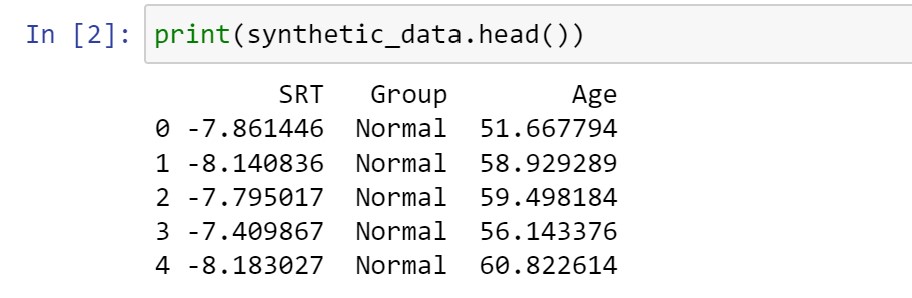
Finally, we converted the NumPy array to a Pandas dataframe called synthetic_data using pd.DataFrame(). This dataframe has three columns: “SRT” for the synthetic SRT data, “Group” for the corresponding group labels, and “Age” for the corresponding age data. We populated the DataFrame with the data from the merged srt_data, groups, and age arrays.

Calculate the Coefficient of Variation using Python & Pandas

We can calculate the coefficient of variation in Python with Pandas using a straightforward approach:

cv = s_data['SRT'].std() / s_data['SRT'].mean() * 100
Code language: Python (python)

In the code above, we use the Pandas functions to calculate the coefficient of variation. First, we call s_data['SRT'].std() to obtain the standard deviation of the SRT data in the DataFrame. Then, we divide this standard deviation by the mean of the SRT data, calculated with s_data['SRT'].mean(). The result provides us with a relative measure of variability.

By multiplying this value by 100, we express the coefficient of variation as a percentage.

Note that we should handle our data’s missing values appropriately. We can use the skipna=True argument in the Pandas functions to exclude missing values when calculating the standard deviation and mean:

cv = s_data['SRT'].std(skipna=True) / s_data['SRT'].mean(skipna=True) * 100Code language: PHP (php)

This method using Python and Pandas allows us to easily compute the coefficient of variation, providing insights into the relative variability of the data. It offers a concise and effective way to analyze data spread and stability. However, the synthetic data contains two groups. Therefore, the next section will cover how to calculate the coefficient of variation by group.
Calculate the Coefficient of Variation by Group in Python with Pandas

Coefficient of Variation by Group in Python

To calculate the coefficient of variation for each group in Python using Pandas, we can leverage the groupby() and agg() functions. Here is an example:

# Calculate coefficient of variation for each group
group_cv = s_data.groupby('Group')['SRT'].agg(lambda x: x.std() / 
                                                      x.mean() * 100).reset_index(name='cv')Code language: Python (python)

In the code above, we use the groupby() function to group the data by the ‘Group’ variable. Then, we apply the agg() function to calculate the coefficient of variation for the ‘SRT’ variable within each group. The lambda function lambda x: x.std() / x.mean() * 100 calculates the coefficient of variation for the ‘SRT’ data within each group.

The resulting group_cv dataframe will contain the coefficient of variation for each group, allowing us to compare the variability between different groups in our data. Here is a post about grouping data with Pandas:

Python Pandas Groupby Tutorial

This approach is handy when we have multiple groups in our dataset and want to analyze and compare the variability within each group separately. It provides a convenient way to examine the coefficient of variation among different groups. Consequently, it allows for gaining insights into the relative variability of the variables within each group. In the following examples, we will use Pandas to calculate the coefficient of variation for all numeric variables.

Calculate the Coefficient of Variation for All Numeric Variables

Here is how we can use the select_dtypes() function to calculate the coefficient of variation for all numeric variables n Python:



# Calculate coefficient of variation for all numeric columns in the dataframe
summary_df = s_data.select_dtypes(include='number').agg(lambda x: x.std() /
                                                                x.mean() * 100).rename('cv').reset_index()Code language: PHP (php)

In the Python chunk above, we use Pandas’ select_dtypes() function to select all numeric columns in the DataFrame s_data. The include='number' argument ensures that only numeric columns are considered for computation.

We then apply the agg() function and a lambda function to calculate each numeric column’s coefficient of variation (cv). The lambda function lambda x: x.std() / x.mean() * 100 computes the coefficient of variation for each column individually.

The resulting summary_df dataframe will contain the coefficient of variation for each numeric column. It provides a convenient and efficient way to summarize and analyze the variability within our dataset.

To handle missing values, you can use the skipna=True argument inside the lambda function:

We can also use, e.g., Pandas to calculate more descriptive statistics in Python. In the following section, however, we will look at a simpler example using a Python list to calculate the coefficient of variation.

Calculate the Coefficient of Variation for a Python List

To calculate the coefficient of variation for a Python list, we can use NumPy. Specifically, we can use the numpy.std() and numpy.mean() functions. Here is an example:

import numpy as np

# Example Python list
data_list = [12, 15, 18, 10, 16, 14, 9, 20]

# Calculate the coefficient of variation
cv = np.std(data_list) / np.mean(data_list) * 100

print(f"Coefficient of Variation: {cv:.2f}%")
Code language: Python (python)

In the code chunk above, we have a Python list called data_list, representing a set of data points. We use np.std(data_list) to calculate the standard deviation of the data and np.mean(data_list) to calculate the mean of the data. Then, we divide the standard deviation by the mean and multiply it by 100 to get the coefficient of variation. The result is printed as a percentage.

Please note that this approach works for a Python list of numeric values. If you have a Pandas dataframe, you can use the same method but access the columns as Pandas Series using df['column_name'] instead of using a Python list directly. See the previous examples in this blog post.

Conclusion

In conclusion, the Coefficient of Variation (CV) is a powerful tool for understanding data variability and making informed decisions. Expressing the standard deviation as a percentage of the mean provides a standardized comparison across different datasets, irrespective of their scales or units.

Throughout this post, we explored the interpretation of CV in the context of Cognitive Hearing Science, which sheds light on speech recognition abilities in noisy environments. We developed synthetic data using Python and Pandas, offering a hands-on understanding of CV’s practical application.

Using Python and Pandas, we learned how to calculate the Coefficient of Variation for individual datasets and multiple numeric variables. This allows us to efficiently summarize and compare data variability among different groups, enhancing our data analysis capabilities.

I encourage you to share this post with fellow data enthusiasts on social media to help them gain insights into the Coefficient of Variation using Python and Pandas. Feel free to comment below for suggestions, requests, or further exploring related topics.

References

Bedeian, A. G., & Mossholder, K. W. (2000). On the use of the coefficient of variation as a measure of diversity. Organizational Research Methods, 3(3), 285-297.

Resources

Explore these valuable Python tutorials to expand your knowledge and skills further: