How to Do the Brown-Forsythe Test in R: A Step-By-Step Example

In this tutorial, you will learn how to do the Brown-Forsythe test in R. This test is great as you can use it to test the assumption of homogeneity of variances, which is important for, e.g. Analysis of Variance (ANOVA).

Outline of the Post
The Hypotheses of the Brown-Forsythe test
Brown-Forsythe Test in R
- Onewaytests
How to Perform Brown-Forsythe test in R: 5 Simple Steps
Conclusion
References & Useful Resources
Additional Resources

Outline of the Post

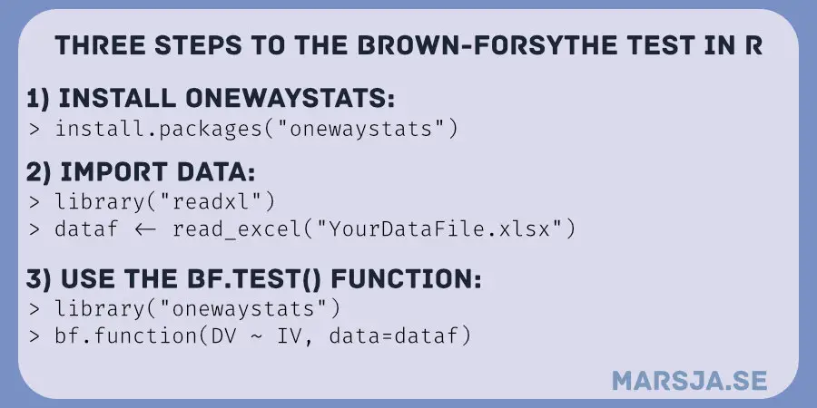
This post is structured as follows. First, we start by answering a couple of questions related to this test. Second, we learn about the hypotheses of the Brown-Forsythe test. This is followed by the most important section, maybe, the 5 steps to performing the Brown-Forsythe test in R. Now, of course, it is possible to do it in fewer steps. Here’s how to carry out the test in three steps, one of which involves installing a package:

The Brown-Forsythe test in R in three steps

What is the Brown-Forsythe test?

This section will give you some brief details on what this test is. As previously mentioned, the Brown Forsythe test is used whenever we need to test the assumption of equal variances. Furthermore, it is a modification of Levene’s test, but the Brown-Forsythe test uses the median rather than the mean (Levene’s). The test is considered a robust test based on the absolute differences within each group from the median group, as previously mentioned. The Brown-Forsythe test is a suitable alternative to Bartlett’s Test for equal variances, as it is not sensitive to a lack of normality and unequal sample sizes. For more information on how the Brown-Forsythe test works, see this article or the resources towards the end of the post.

How can I Carry out the Brown-Forsythe test in R?

You can perform the Brown-Forsythe test using the bf.function() from the R package onewaytests. For example, bf.function(DV ~ IV, data=dataFrame) will successfully test the dependent variable DV and the groups IV, in the dataframe dataFrame.

In the next section, you will learn the hypotheses of the Brown-Forsythe test. Knowing the hypothesis will make the interpretation of the results easier.

The Hypotheses of the Brown-Forsythe test

When carrying out the Brown-Forsythe test using R, we are testing the following two hypotheses:

H^₀: The population variances are equal.
H_A: The population variances are not equal.

Therefore, as we will see when going through the example, we don’t want to reject the null hypothesis (H0). In the next section, you will get a brief overview of one of the R packages that can be used to perform the test.

Brown-Forsythe Test in R

Now, R is, as you may know, an open-source language. This means that more packages probably make it possible for us to do the Brown-Forsythe test in R. In this post, however, we will only use one package: the onewaytests. In the next section, you will get brief information about this package.

Onewaytests

The Onewaytests package is more focused on carrying out one-way tests. Using this package, we can carry out one-way ANOVA, Welch’s heteroscedastic F test, Welch’s heteroscedastic F test with trimmed means and Winsorized variances, Brown-Forsythe test, and Alexander-Govern test, James second-order test to name a few. The function bf.test() is, of course, of interest for this blog post. In the next section, you will learn how to carry out the Brown-Forsythe test in R using the onewaystats package.

See also these posts about non-parametric tests:

How to do a Kruskal-Wallis Test in R

How to Perform Brown-Forsythe test in R: 5 Simple Steps

We are now ready to carry out the Brown-Forsythe test in R. In the first step, we will install the onewaytests package. Note that if you already have this package installed, you can jump to the next step (importing your data).

Step 1: Installing the onewaytests Package

Now, you may already know how to install R-packages, but here’s how we install the onewaytests package:

install.packages("onewaytests")Code language: R (r)

Note, we are, in step three, also going to summarize data to calculate variance, for each group, using dplyr. Moreover, we will import the example dataset using the readxl package. Both packages are part of the Tidyverse package. Therefore, to fully follow this post, install the TIdyverse package (or just dplyr, of course), as well:

install.packages(c("onewaytests", "tidyverse"))Code language: R (r)

The above code will install both onewaytests and Tidyverse. If you, on the other hand, only want to install dplyr and readxl (for reading Excel files) you can remove “tidyverse” and add “dplyr” and “readxl”. Just follow the syntax above. Now, Tidyverse comes with a lot of great packages. For example, you can use dplyr to rename columns, count the number of occurrences in a column, stringr to merge two columns in R.

In the next step, we will use the readxl package to import the example dataset.

Step 2: Import your data into R.

Here’s how we read an Excel file in R using the readxl package:

library(readxl)

dataFrame <- read_excel('brown-forsythe-test-in-R-example-data.xlsx')Code language: R (r)

First, before going on to the next step, we can explore the data frame a bit. For example, we can get the first six rows:

head(dataFrame)Code language: R (r)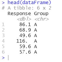

First 5 rows of example data to ise the brown-forsythe test

As we can see, only two variables exist in this example data. First, we have the column “Group”, in which we find the different treatment groups (“A”, “B”, and “C”). If we want to see what data type we can type this:

str(dataFrame)

Now, we see that Group is factor and Response is numeric (i.e., num). In the next, section, we will have a visual look at the variance of Response, in each group.

It is also possible to convert a matrix to a dataframe in R or convert a list to dataframe in R. If your data is stored in any of these two data types, of course. In the next step, you will learn how we can explore data. If you already know this, you can skip to the fourth step: carrying out the Brown-Forsythe test using the R package onewaystats.

Step 3: Exploring the Data by Visualizing and Calculating Variance

As you may know, there are many different ways to visualize data in R. Here we will make use of the boxplot() function which will give us an idea of whether the variances are equal across the groups, or not. Here’s how to create a boxplot:

boxplot(Response ~ Group, data = dataFrame)Code language: R (r)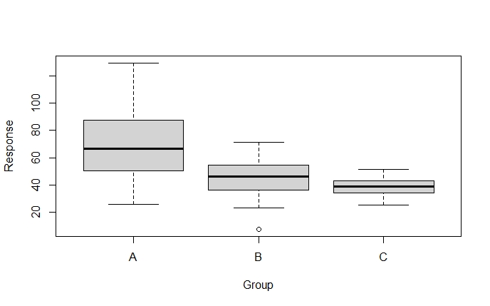

When inspecting the boxplots, it sure looks like the variances are different for the treatment groups. We can also calculate the variance, by group, using dplyr:

library(dplyr)
dataFrame %>%
  group_by(Group) %>%
  summarize(Variance=var(Response)) Code language: R (r)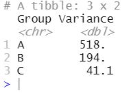

checking the variance before doing the brown forsythe test in R — Variance

Note, you can see the following two posts if you need to calculate other summary statistics as well:

Now, judging from the image above, it also looks like we have different variances in the different treatment groups. In the next step, however, we will use the bf.test() function to carry out the Brown-Forsythe test testing the null hypothesis that the variances are equal.

Step 4: Carry out the Brown-Forsythe Test

Here’s how you can perform the Brown-Forsythe Test in R:

library(onewaytests)

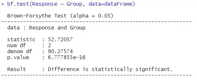
bf.test(Response ~ Group, data = dataFrame)Code language: R (r)

In the code chunk above, we used the bf.test() function (onewaytests package) to carry out the Brown-Forsythe test. Note how we used the formula as the first argument. This would be the exact same formula you would use performing ANOVA in R. Here’s the output from the function:

In the next section, we will learn how to interpret the results from the test.

Step 5: Interpreting the Results

Interpreting the Brown-Forsythe test is quite simple. Remember that we had the null hypothesis that the variances are equal across the groups. Therefore, if the p-value is under 0.05, we reject the null hypothesis and conclude that the data does not meet the assumption of variance homogeneity.

In our example, the null hypothesis is rejected. However, if the p-value had been above 0.05, we would not reject the null hypothesis. In this case, we can safely carry out e.g. one-way ANOVA.

If your data is violating the assumption of homogeneity but is normally distributed, you should carry on with Welch’s ANOVA, which also can be carried out in R. We can also use a residual plot created in R to guide our decision.

Conclusion

In this blog post, you have learned how to carry out the Brown-Forsythe test of homogeneity of variances in R. Specifically, you have learned, step-by-step, how to carry out this test. First, you learned how to install an R package enabling the Brown-Forsythe test in R. Second, you imported example data and, third, explored the data. Finally, you learned how to carry out the test using the bf.test() function. There are probably other packages and functions that enable us to carry out this test of equal variances. Please leave a comment below, if you know any other packages or functions that we can use to do the Brown-Forsythe test in R. You are, of course, also welcome to suggest what I should cover in future blog posts, correct any mistakes in my blog posts, or just let me know if you found the post helpful. That is, I encourage you to comment below!

References & Useful Resources

Here are some references and useful resources that you might find helpful on the topic:

Additional Resources

Here are some other blog posts found on this blog that you might find useful.