Durbin Watson Test in R: Step-by-Step incl. Interpretation

This blog will teach you how to carry out the Durbin-Watson Test in R. Have you ever run a linear regression model in R and wondered if the model’s assumptions hold? One common assumption of a linear regression model is the independence of observations, which means that the residuals (the differences between predicted and actual values) should not be correlated. However, this assumption may be violated in some cases, leading to biased estimates and incorrect conclusions.

To check for autocorrelation, we can use the Durbin-Watson test, which is a statistical test to determine if there is evidence of autocorrelation in the residuals of a linear regression model.

Outline

We will begin by discussing the hypotheses of the Durbin-Watson test and the requirements for carrying out the test in R. We will provide examples of how the Durbin-Watson test can be applied in different fields, such as data science, psychology, and hearing science.

Next, we will introduce you to the syntax of the dwtest() and durbinWatsonTest() functions, two functions that can be used to carry out the Durbin-Watson test in R. We will also provide you with an example data set to help you understand how to use these functions.

We will then guide you through the steps to carry out the Durbin-Watson test in R, including how to fit a linear regression model, install and load the necessary packages, run the test, and interpret the results. Moreover, we will also discuss what to do if autocorrelation is detected and alternative methods for testing for autocorrelation.

By the end of this blog post, you will have a good understanding of how to check for autocorrelation in a linear regression model using the Durbin-Watson test in R. Whether you are a data scientist, psychologist, or hearing scientist, this post will equip you with the knowledge and skills to ensure that your linear regression models are sound and valid.

Durbin Watson Test

We can use the statistical test Durbin-Watson test to detect the presence of autocorrelation in regression models. Autocorrelation refers to the presence of correlation between the error terms of a regression model, which can occur when the data points are not independent of each other. The Durbin-Watson test can be used to test for autocorrelation in various fields, including data science, cognitive psychology, and hearing science.

Hypotheses

The null hypothesis for the Durbin-Watson test is that no autocorrelation exists in the model’s residuals. The alternative hypothesis is that the residuals have positive or negative autocorrelation.

The test statistic for the Durbin-Watson test ranges from 0 to 4, with a value of 2 indicating no autocorrelation. A less than 2 indicates positive autocorrelation, while a value greater than 2 indicates negative autocorrelation. A value of 0 indicates perfect positive autocorrelation, and 4 indicates perfect negative autocorrelation.

Data Science Example

In data science, the Durbin-Watson test is used to evaluate the presence of autocorrelation in time series data. Time series data are points collected over time, such as stock prices or weather patterns. Autocorrelation in time series data occurs when the error terms of a regression model are correlated with previous error terms, indicating that the data points are not independent of each other. This can lead to biased estimates and incorrect statistical inferences. Data scientists can use the Durbin-Watson test to identify and correct autocorrelation in their time series models.

For example, a data scientist may analyze stock prices to predict future market trends. If there is autocorrelation in the data, the model may incorrectly predict future prices, leading to significant financial losses. Using the Durbin-Watson test, the data scientist can detect and correct for any autocorrelation, improving the accuracy of their model.

Psychology Example

In cognitive psychology, the Durbin-Watson test is used to analyze data from experiments that involve repeated measurements of the same participants. Autocorrelation in this context can occur when the error terms of a regression model are correlated with previous error terms, indicating that the participant’s responses are not independent of each other. This can lead to biased estimates of the effects of independent variables and incorrect statistical inferences. Cognitive psychologists can use the Durbin-Watson test to identify and correct autocorrelation in their models.

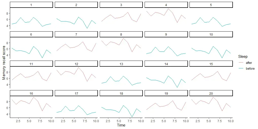
For example, a cognitive psychologist may conduct an experiment to test the effects of sleep on memory. Participants are tested on their memory recall immediately after learning a list of words and again after a night of sleep. Autocorrelation in this context may occur if the error terms of the regression model are correlated with previous error terms, indicating that the participants’ memory recall is not independent of each other. Using the Durbin-Watson test, cognitive psychologists can detect and correct for any autocorrelation, improving the accuracy of their results.

Hearing Science Example

In hearing science, the Durbin-Watson test can analyze data from experiments involving repeated auditory stimuli measurements. Autocorrelation in this context can occur when the error terms of a regression model are correlated with previous error terms, indicating that the participant’s responses to auditory stimuli are not independent of each other. This can lead to biased estimates of the effects of auditory stimuli and incorrect statistical inferences. Hearing scientists can identify and correct autocorrelation in their models using the Durbin-Watson test.

For example, a hearing scientist may be conducting an experiment to test the effects of background noise on speech perception. Participants are tested on their ability to identify spoken words in background noise. Autocorrelation in this context may occur if the error terms of the regression model are correlated with previous error terms, indicating that the participant’s responses to auditory stimuli are not independent of each other. Using the Durbin-Watson test, the hearing scientist can detect and correct for any autocorrelation, improving the accuracy of their results.

What package do you need for a Durbin-Watson test in R?

You can carry out a Durbin-Watson test in R using the lmtest package or the car package. Both packages provide functions for running the Durbin-Watson test on a linear regression model in R.

Requirements for Carrying out the Durbin-Watson test in R

A few requirements need to be met to carry out the Durbin-Watson test in R. First, we need a model (e.g., a linear regression model) we want to test for autocorrelation. We could, e.g., fit the model using the lm() function in R. The model should have at least one independent variable and one dependent variable. Once we have a fitted model, we can use the dwtest() function in the lmtest package to carry out the Durbin-Watson test.

The dwtest() the function takes a fitted linear regression model as an input and returns a p-value that indicates the test’s significance. If the p-value is less than the significance level (typically 0.05), we can reject the null hypothesis and conclude that there is evidence of autocorrelation in the residuals.

In addition to the lmtest package, we can also use the durbinWatsonTest() function in the car package to carry out the Durbin-Watson test. The durbinWatsonTest() function also takes a fitted linear regression model as an input and returns a test statistic and a p-value.

Syntax of the dwtest()

The dwtest() function from the lmtest package can be used to perform the Durbin-Watson test in R on a linear regression model. The syntax for the function is as follows:

Arguments:

Here are the arguments briefly explained:

formula: This is the formula for the regression model you want to test for autocorrelation. It should be in the form of response ~ predictor1 + predictor2 + .... It can also contain a lm() object that you have fitted.
order.by: This optional argument allows you to specify a variable to order the data by before running the test. This is useful if you suspect that there may be some other variable that is causing the autocorrelation in the data.
alternative: This argument specifies the alternative hypothesis for the test. It can take on one of three values: “greater”, “two.sided”, or “less”. If you think the autocorrelation is positive, you should set this to “greater”. If you think it is negative, you should set it to “less”. If you don’t know, leave it at the default value of “two.sided”.
iterations: This is the number of iterations used in the Monte Carlo simulation to compute the p-value. The default value is 15, which is generally sufficient for most purposes. However, you may need to increase this value if you have a large dataset or the autocorrelation is very strong.
exact: This optional argument allows you to specify whether to use an exact test instead of the Monte Carlo simulation. This is generally unnecessary but useful if you have a small dataset.
tol: This is the tolerance level used in the test. The default value is 1e-10, which is generally sufficient for most purposes. However, if you have a very large dataset or if the autocorrelation is very weak, you may need to decrease this value.
data: This dataframe contains the variables used in the regression model.

In the next section, we will have a look at the durbinWatsonTest() function from the car package.

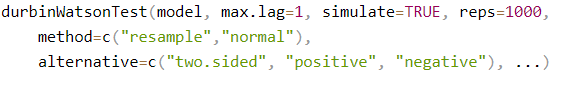
Syntax of the durbinWatsonTest()

The durbinWatsonTest() function from the car package is used to perform a Durbin-Watson test on a linear regression model. The function takes several arguments:

Arguments

Again, here are the arguments briefly explained.

model: The fitted linear regression model object.
max.lag: The maximum lag to test for autocorrelation. By default, the function tests for first-order autocorrelation.
simulate: A logical value indicating whether to use a simulation-based approach to calculate the p-value. If simulate=TRUE, the function performs a Monte Carlo simulation to estimate the p-value. If simulate=FALSE, the function uses an approximation to the distribution of the test statistic.
reps: The number of Monte Carlo replications to use if simulate=TRUE.
method: The method to use for calculating the p-value if simulate=TRUE. The options are "resample" (default) and "normal". The "resample" method is a permutation-based approach that resamples the model’s residuals to simulate the null distribution. The "normal" method assumes that the residuals are normally distributed and uses this assumption to calculate the p-value.
alternative: The alternative hypothesis to test. The options are "two.sided" (default), "positive", and "negative".
...: Additional arguments to be passed to the summary() function.

In the next section, we will generate fake data to practice running the Durbin-Watson test.

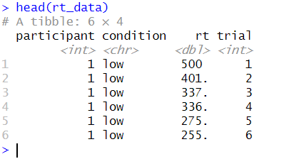
Example Data

Here is some example data to practice the Durbin-Watson test in R:

library(tidyverse)

# Define the number of participants, conditions, and trials per condition
n_participants <- 50
n_conditions <- 2
n_trials <- 10

# Define the autocorrelation coefficient (rho)
rho <- 0.8

# Generate the reaction time data
rt_data <- tibble(
  participant = rep(1:n_participants, each = n_conditions * n_trials),
  condition = rep(rep(1:n_conditions, each = n_trials), times = n_participants),
  rt = unlist(
    lapply(1:n_participants, function(p) {
      lapply(1:n_conditions, function(c) {
        x <- seq(from = 500, to = 700, length.out = n_trials)
        for (i in 2:n_trials) {
          x[i] <- rho * x[i - 1] + abs(rnorm(1, mean = 0, sd = 50))
        }
        # x[x < 200] <- 200
        return(x)
      })
    })
  )
)

rt_data <- rt_data %>% 
  mutate(condition = if_else(condition == 1, "low", "high"),
         trial = rep(seq(1, 20), n_participants))Code language: R (r)

In the code chunk above, we generated example data using the tidyverse package in R. The data consists of reaction times from 50 participants who performed two conditions (high vs. low load) with ten trials per condition. Next, we set the autocorrelation coefficient (rho) to 0.8 to ensure a correlation between consecutive reaction times within each condition. Using the seq() function, we generated the reaction times to create a sequence from 500 to 700 with ten values. Then, the autocorrelation coefficient was applied to create a correlated sequence using a for loop. Here we also used the abs() function to take the absolute value in R. Moreover, any values under 200 were replaced with 200 to ensure no values under 200 ms.

Now, we are ready to go to the next section and carry out the Durbin-Watson test in R.

How to Carry out the Durbin-Watson Test in R

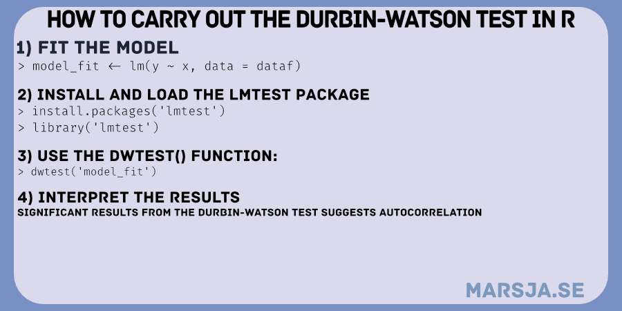
To carry out the Durbin-Watson test in R, you can follow these steps:

Fit a linear regression model using the lm() function in R.
Install and load the lmtest package or the car package, which both contain the Durbin-Watson test function.
Use the dwtest() function from the lmtest package or the durbinWatsonTest() function from the car package to perform the Durbin-Watson test.
Interpret the results of the Durbin-Watson test by examining the test statistic and the associated p-value.

1. Fit a Linear Regression Model in R

Here is how to fit a linear regression model in R using the lm() function:

# Fit a linear regression model
rt_model <- lm(rt ~ trial, data = rt_data)Code language: R (r)

In the code chunk above, we fitted a linear regression model using the lm() function in R. We used the model formula rt ~ trial to specify that we want to model the response variable rt as a function of the predictor variable trial. Here, rt is the variable containing the reaction time data, and trial is the variable containing the trial numbers.

Finally, we used the data argument to specify the dataframe containing the variables used in the model. Here, the data frame is rt_data, which we previously generated.

Probit Regression in R: Interpretation & Examples

2. Install and load the lmtest package or the car package

Here is how we can install and load the lmtest package in R:

install.packages('lmtest')
library('lmtest')Code language: R (r)

Alternatively, we can use the durbinWatsonTest() from the car package. In the following section, we are ready to run the Durbin-Watson test in R. Note that we do not have to install the car package.

3. Run the Durbin-Watson Test in R

Here is an example code chunk that demonstrates how to carry out the Durbin-Watson test in R:

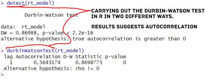
# Perform the Durbin-Watson test
dwtest(rt_model)Code language: R (r)

Alternatively, we can use the durbinWatsonTest() from the car package to carry out the Durbin-Watson test:

# Carry out the Durbin-Watson test
durbinWatsonTest(rt_model)Code language: PHP (php)

In the following section, we are going to interpret the results. Note that this is just example data; we would most likely not analyze a similar actual data set like this.

durbin-watson test in R using lmtest and car. — Durbin-Watson Results in R

4. Interpret the Results from the Durbin-Watson Test in R

In the Durbin-Watson test output above, we performed a test for first-order autocorrelation in the residuals of the linear regression model rt_model that was fit to the rt_data. Remember, the null hypothesis for the test is that there is no first-order autocorrelation in the residuals, i.e., the errors are independent. On the other hand, the alternative hypothesis is positive autocorrelation in the residuals.

The Durbin-Watson test statistic (DW) is a value between 0 and 4 that measures the degree of autocorrelation in the residuals. The value DW is interpreted as follows:

If DW = 2, there is no autocorrelation in the residuals.
If DW < 2, there is positive autocorrelation in the residuals.
If DW > 2, there is negative autocorrelation in the residuals.

In our case, the value of DW is 0.89, which is less than 2. This suggests positive autocorrelation in the model’s residuals, which supports the alternative hypothesis.

The p-value for the test is less than 2.2e-16, which is smaller than the conventional level of significance (e.g., 0.05). This indicates strong evidence against the null hypothesis of no autocorrelation in the residuals. Therefore, we can reject the null hypothesis in favor of the alternative hypothesis and conclude that there is positive autocorrelation in the residuals.

We can see that the results from the Durbin-Watson test output suggest positive autocorrelation in the residuals of the linear regression model rt_model. This implies that the errors are not independent and may violate the assumption of independent errors in the linear regression model. If this were real data, we would have to be cautious as this can lead to biased parameter estimates and incorrect inference. Therefore, it is important to account for autocorrelation in the residuals when analyzing the data or to use a different model that allows for autocorrelated errors.

What to do when the Durbin-Watson test in R is Significant?

Suppose the results from the Durbin-Watson test are significant, indicating a presence of autocorrelation in the residuals of a linear regression model. In that case, several steps can be taken:

Model modification: Autocorrelation in the residuals can indicate some important information that the current model is not capturing. One possible solution is to modify the model to include additional predictors or interactions between predictors that might account for autocorrelation.
Use a different regression method: If autocorrelation in the residuals persists even after model modification, it might be necessary to use a different regression method that can handle autocorrelation, such as generalized least squares (GLS) or autoregressive integrated moving average (ARIMA) models.
Use a different type of data: If autocorrelation cannot be eliminated using the above methods, it might be necessary to use another type of data collection to reduce the potential for autocorrelation. For example, repeated measures designs or time-series data collection can help to reduce autocorrelation.
Report the results: Regardless of whether or not autocorrelation can be eliminated, it is important to report the results of the Durbin-Watson test and any subsequent modifications to the model in any publications or reports. This allows readers to interpret the results and understand any potential analysis limitations.

Alternative Methods for Testing for Autocorrelation

Finally, here are some alternatives to the Durbin-Watson test:

Breusch-Godfrey Test: This test is an extension of the Durbin-Watson test and can be used to test for higher-order autocorrelation. The null hypothesis is no autocorrelation, and the alternative hypothesis is the presence of autocorrelation.
Cochrane-Orcutt Procedure: This method is used when the errors have first-order autocorrelation. It involves transforming the variables and fitting a new model to the transformed data. The Durbin-Watson test can be used to test for autocorrelation in the transformed errors.
The generalized Method of Moments (GMM) estimates the model’s parameters using instrumental variables. We can use it to correct autocorrelation in the errors.
Newey-West Estimator: This is a robust method that can be used to estimate the standard errors of the coefficients in autocorrelation. It involves adjusting the standard errors using a correction factor based on the lagged values of the residuals.

Of course, you need to check other linear (regression) model assumptions. For example, you can look at the possible outliers by making a residual plot in R and testing for normality in R.

Conclusion: Durbin-Watson Test in R

In this blog post, you have learned about the Durbin-Watson test, a statistical method used to examine autocorrelation in regression models. You have seen how the test is based on two hypotheses, which can help you determine whether there is evidence of positive or negative autocorrelation in your data.

We examined three examples of how the Durbin-Watson test can be used in different fields, including Data Science, Psychology, and Hearing Science. We also discussed the requirements for carrying out the test in R and provided step-by-step instructions on using both the lmtest and car packages to perform the test.

Moreover, we have explained the syntax of the dwtest() and durbinWatsonTest() functions and demonstrated how to interpret the results. Additionally, we have shown how to correct autocorrelation in your data and discussed alternative methods for testing for autocorrelation.

We hope that this blog post has been informative and helpful. If you enjoyed reading it or found it useful, please consider sharing it on social media or citing it in your work. If you have any comments or questions, please leave them below. I appreciate any feedback and would be happy to hear from you.