In this post, we will learn how to transform data from wide to long in R. Wide-to-long format conversion is often an important data manipulation technique in data analysis. In R, we can use many packages and their functions to transform data from a wide to long format. These functions include the tidyr package’s pivot_longer() and the reshape2 package’s melt(). The transformation is essential when dealing with data with variables organized in a wide format, making it difficult to analyze or visualize using certain statistical analysis techniques or visualization libraries.
In cognitive hearing science and psychology, for example, wide-format data is commonly used to store data obtained from multiple hearing or cognitive tests, such as multiple assessments of participants’ hearing and cognitive abilities. However, many analysis packages in R afex require data to be in long format. In addition, plotting packages, such as ggplot2, also require data in long format for certain types of plots.

Table of Contents
- Outline
- Wide format
- Long format:
- Wide vs. Long Format
- R Packages for Melting Data from Wide to Long
- Requirements
- Example Data
- Syntax of pivot_longer()
- The Syntax of the melt() Function
- Wide to Long in R using pivot_longer
- R Wide to Long using melt from reshape2
- pivot_longer() vs. melt() for Reshaping from Wide to Long in R
- Conclusion: Wide to Long in R
- Resources
Outline
The tidyr package’s pivot_longer() function allows for efficient data conversion from wide to long format by gathering columns based on a set of rules. This function is handy when working with datasets with multiple sets of variables that need to be gathered separately. In contrast, the reshape2 package’s melt() function creates a long format data frame by stacking all columns in a wide format dataset into a single column, making it easier to use with other R packages that require long format data.
In this tutorial, we will demonstrate how to transform wide format data to long format using pivot_longer() from the tidyr package and melt() from the reshape2 package. We will use an example dataset of participants’ hearing and cognitive test scores to show how the two functions work. The tutorial will include two examples of using pivot_longer() and one example of using melt(), highlighting the similarities and differences between the two functions. The examples will show how the data changes from a wide to long format.
Wide format
Wide format is a common way to store data in tables. In wide format, each variable is stored in its column, and each observation is stored in its row. This format is useful when dealing with data with a few variables but many observations. For example, in psychology, a study might have a variable for each question on a survey. Here, the responses to those questions might be stored in a wide format.
Here is an example of how data might be stored in wide format in R. Imagine that we conducted a study on the effects of caffeine on cognitive performance. In this study, we asked participants to complete a survey before and after drinking coffee. In wide format, our data might look like this:
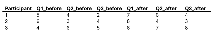
In this example, we have three variables (Q1, Q2, and Q3) and six observations (two for each participant). While this format is easy to understand, it can be difficult to analyze because the data is spread across many columns.
Long format:
Long format is another method for storing data in tables. In long format, each observation is stored in its row, and each variable is stored in its column. This format is useful when dealing with data that has a large number of variables but a small number of observations. For example, in psychology, a study might have many variables that measure different aspects of a person’s personality. The responses to those variables might be stored in a long format.
Here is an example of how data might be stored in long format in R. Imagine that we conducted a study on the effects of mindfulness meditation on well-being. Here we asked participants to complete a questionnaire with multiple questions. In long format, our data might look like this:
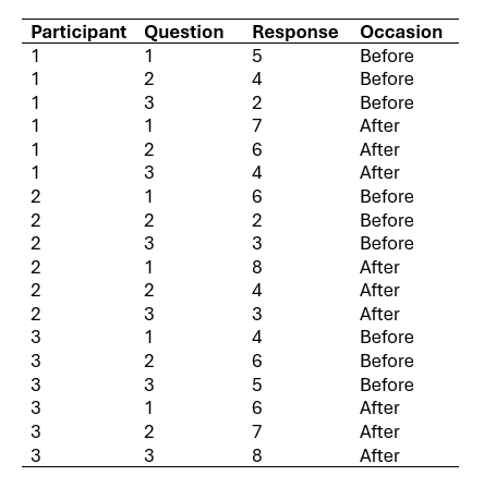
In this example, we have many variables (each question is a variable) and only three observations. While this format is more challenging to understand at first glance, it is often easier to analyze because the data is organized into a single column.
The long format is particularly useful when dealing with data that has multiple observations for each subject or with data that has many variables with similar meanings. The long format is also useful for storing data in a way that facilitates easier analysis using specific statistical methods and packages.
For example, when using the R package tidyverse, many of the functions work best with data in long format. In addition, when using analysis of variance (ANOVA) or linear regression, long format can make it easier to perform the analysis. In particular, when dealing with repeated measures or within-subjects designs.
Wide vs. Long Format
There are exceptions to the rule mentioned above (that long format is often preferred). In some cases, wide format may be preferred. For instance, when dealing with data that has a small number of variables and a large number of observations. Additionally, some statistical methods and packages may require data to be in a specific format. Therefore, it is always essential to consult the documentation or consult with a statistician before determining the format of your data.
In summary, while long format is often useful for storing and analyzing data in certain situations, it’s important to consider the specific needs of your analysis and consult with experts when making decisions about data format.
R Packages for Melting Data from Wide to Long
In R, many packages can transform data from wide to long format. Here are a few examples:
- tidyr is a package within the tidyverse that provides functions for reshaping data. The pivot_longer function can be used to convert data from wide to long format in R. We can use this function to specify which columns should be converted into “long” format. Additionally, we can specify the names of the resulting columns.
- reshape2 is another package that provides functions for reshaping data. The
meltfunction can be used to convert data from wide to long format. This function allows you to specify which columns should be converted into a “long” format. Of course, we can specify the names of the resulting columns. - data.table is a package that provides high-performance data manipulation tools. The
meltfunction in data.table is another R function that we can use to convert wide to long format. This function is similar to themeltfunction in the reshape2 package. - reshape is an older package that provides functions for reshaping data. The
meltfunction in reshape can be used to convert data from wide to long format. This function is similar to the “melt” function in reshape2.
When using these packages, it is essential to note that converting data from a wide to a long format syntax can vary slightly between packages. Additionally, some packages may offer more advanced functionality. For example, some can reshape data based on regular expressions or other patterns. See an example of how to transition from a wide to a long format when reporting correlation results in an APA table.
In general, however, these packages provide powerful tools for transforming data between wide and long formats, which can be a key step in preparing data for analysis. This post will use the tidyr and reshape2 packages to transform data from wide to long format in R.
Requirements
If you want to learn how to convert your data from wide to long format using R, dplyr, and tidyr there are a few things you should know before getting started. First, you need some basic knowledge of R and how to read data. It would be best if you were comfortable using, e.g., the read.csv() function to read your data from a CSV file or a similar format. Of course, in this tutorial, we are working with example data.
Once you have your data loaded into R, you will need to have the dplyr and tidyr packages installed. These packages are part of the larger tidyverse ecosystem and provide tools for working with tidy data. You can install these packages using the install.packages() function in R. Here is how to install a package in R:
install.packages('tidyverse')Code language: R (r)In addition to these basic steps, you may need to perform some data cleaning or manipulation before pivoting your data. For example, you may need to rename your column names or filter out missing values. However, these steps depend on your data’s specific structure and content. In the next section, we will generate some example data. Note that for, e.g., security reasons, make sure to keep an updated version of R (i.e., the latest stable version).
Example Data
Here is an example dataset we can use to practice converting from wide to long format in R. Imagine that we have data on participants’ performance in a hearing and cognition study. We measured their scores on two different hearing tests, as well as their scores on two different cognitive tests. The dataset is called hearing_cognition_scores.
library(dplyr)

# Generate example data
hearing_cognition_scores <- data.frame(
  participant_id = 1:20,
  hearing_HINT1 = sample(1:10, 20, replace = TRUE),
  hearing_HINT2 = sample(1:10, 20, replace = TRUE),
  cognitive_Stroop1 = sample(1:100, 20, replace = TRUE),
  cognitive_Stroop2 = sample(1:100, 20, replace = TRUE)
)Code language: R (r)
In this dataset, each row corresponds to a single participant, and there are four variables: participant_id, hearing_test_1, hearing_test_2, cognitive_test_1, and cognitive_test_2. The variables hearing_test_1 and hearing_test_2 represent scores on the two different hearing tests, while cognitive_test_1 and cognitive_test_2 represent scores on the two different cognitive tests. In the next section, before working with the data, we will look at the syntax of the pivot_longer() function.

Syntax of pivot_longer()
As you may know now,pivot_longer()is a function in the tidyr package that we can use to transform wide data into long format. The first argument, data, is the input data frame.
We can use the second argument, cols, to specify which columns to pivot. It can be a numeric vector or a selection helper, such as starts_with(), ends_with(), or contains(). In a way, it works similarly to the select() function from dplyr.
Additional arguments include cols_vary, which determines how to treat columns with different lengths, and names_to, which specifies the name of the new column containing the previously wide column names. We can use the names_prefix and names_sep to remove a prefix from the variable names or split them into multiple columns using a separator.
names_pattern allows for specifying a regular expression pattern to match and split variable names. values_to specifies the name of the new column containing the previously wide cell values. Other optional arguments include values_drop_na to remove missing values, values_ptypes to specify the data type of the new column containing cell values, and values_transform to apply a transformation function to the cell values.
To summarize, pivot_longer() is a versatile function that can handle various types of data transformations flexibly. In the next section, before transforming data from wide to long in R using pivot_longer() we will look at the syntax of the melt() function.
The Syntax of the melt() Function
We can also use the melt() function in R to reshape a dataset from a wide format to a long format. It takes in the data set that needs to be reshaped as its first argument. The additional arguments are passed to or from other methods and are optional.
We can, for example, use the na.rm argument to remove missing values from the data set. If set to TRUE, any missing values are removed, resulting in a smaller data set. If set to FALSE, the missing values are preserved, and the resulting data set will be the same size as the original data set.
Moroevoer, we can use the value.name argument to specify the name of the new variable that will be created to store the values of the original dataset. By default, the new variable’s name is set to “value”. However, this argument can specify a different name for the new variable.
The ... argument allows for additional arguments to be passed to or from other methods. These arguments will depend on the specific implementation of melt() being used, and may not be necessary in all cases.
To summarize, the melt() function is a useful tool for reshaping a dataset from a wide format to a long format, allowing for easier analysis and visualization.
Wide to Long in R using pivot_longer
In this section, we are going to use pivot_longer() in two examples to convert from long to wide in R.
Example 1:
Here is how to transform data from wide to long format in R using pivot_longer:
library(tidyr)

# Convert wide to long format
hearing_cognition_long <- pivot_longer(hearing_cognition_scores,
                                       cols = -participant_id,
                                       names_to = c("test_type", "Test"),
                                       names_sep = "_",
                                       values_to = "Score")Code language: R (r)
In the code chunk above, we use the pivot_longer() function from the tidyr package to convert a wide data set to a long format. The data set used in this example is called hearing_cognition_scores, and it has a column for participant IDs and two columns each for hearing and cognitive test scores. The goal is to transform the data set from a wide to a long format. Now, we can, for example, analyze the data more easily.
To achieve this, we pass the hearing_cognition_scores data frame to the pivot_longer() function, along with several arguments. The cols argument specifies which columns to pivot. In this case, we want to pivot all columns except for the participant_id column, so we use -participant_id.
We use the names_to argument to specify the new names for the columns created during the pivot. Next, we want to split the original column names into two new columns, one for the type of test (test_type) and one for the test number (Test).
Using the names_sep argument, we specify the character separating the test_type and Test columns in the original names. In our example, the separator is an underscore (_). However, it could be another character, such as “.”.
Finally, we use the values_to argument to specify the name of the new column containing the values previously in the hearing and cognitive test score columns. In this case, we use Score.
Example 2:
In this example, we will use pivot_longer() to gather both the hearing and cognitive test data into a single column, and use separate() to split the test data into two separate columns based on the test type.
# Load required packages
library(dplyr)
library(tidyr)

# Pivot the data to a long format
hearing_cognition_long <- hearing_cognition_scores %>%
  pivot_longer(
    cols = starts_with("hearing_") | starts_with("cognitive_"),
    names_to = c("test_type", "test_number"),
    names_pattern = "(\\D+)(\\d+)",
    values_to = "score"
  ) %>%
  # Split test_type column into two separate columns
  separate(test_type, c("test_domain", "test_name"), sep = "_")Code language: R (r)
In the code chunk above, we start by loading the required packages for our analysis, which are dplyr and tidyr. Next, we use the %>% operator from the dplyr package to pipe the hearing_cognition_scores data frame into the pivot_longer() function. We specify the columns to pivot using the cols argument and use the starts_with() function to select all columns that start with either hearing_test or cognitive_test. Here we make use of “|” which is or in R.
We then use the names_to argument to split the column names into two parts, test_type and test_number. The names_pattern argument uses regular expressions to specify the pattern for the split. In this case, we use (\\D+)(\\d+), which matches any non-digit characters followed by one or more digits.
The values_to argument specifies the column name where the values will be stored, in this case “score”. We then use the %>% operator again to pipe the output of pivot_longer() into the separate() function, which is used to split the test_type column into two separate columns. We use the sep argument to specify the separator as an underscore _.
Finally, we assign the result to a new data frame called hearing_cognition_long.
R Wide to Long using melt from reshape2
In this section, we are going to use the R package reshape2 to transform data from wide to long.
Example:
Here is to convert data from wide to long using the melt() function:
# Load required package
library(reshape2)
# Convert wide to long format
hearing_cognition_long <- melt(hearing_cognition_scores,
id.vars = "participant_id",
variable.name = "test_type",
value.name = "Score") %>%
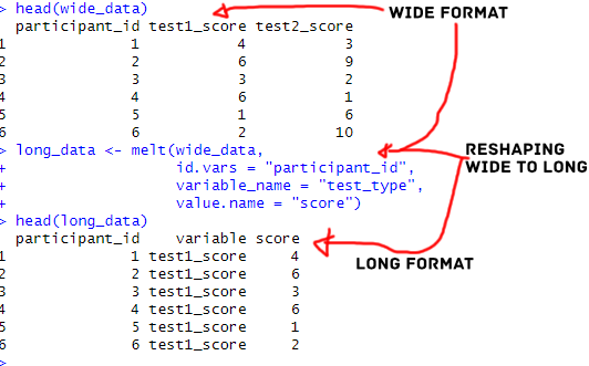
separate(test_type, into = c("test_domain", "test_number"), sep = "_")Code language: R (r)In the code chunk above, we load the reshape2 package to work with our data. We then use the melt() function to convert our wide format hearing_cognition_scores data into a long format hearing_cognition_long data. The id.vars argument specifies the column to use as the identifier variable, in this case, the participant_id column. The variable.name argument specifies the column name that will contain the variable names in the melted data, which is test_type in this case. The value.name argument specifies the name of the column that will contain the variable values in the melted data, which is Score.
After melting the data, we use the %>% pipe operator to pass the melted data to the separate() function. We use the test_type column as the column to separate, and we separate it into two new columns, test_domain and test_number, using the into argument. The sep argument specifies the character to separate the test_type column by, which is the underscore character in this case.
This code achieves the same result as the previous code chunks that used the pivot_longer() function from the tidyr package. However, in this case, we used the melt() function from the reshape2 package to convert the data from wide to long format and then used the separate() function to split the test_type column into two new columns.
pivot_longer() vs. melt() for Reshaping from Wide to Long in R
As you now know, pivot_longer() is part of the tidyr package. The function offers considerable flexibility for reshaping data. One of its main advantages is its ability to handle multiple columns at once. We have seen that this function can be useful when many columns need to be melted. Additionally, it allows users to specify column types and even perform operations on the melted data as part of the same pipeline. Another benefit is that pivot_longer() is generally faster than melt() for large datasets.
On the other hand, melt() from the reshape2 package is a simpler function that may be more intuitive for beginners. It is particularly useful for melting data that has a specific structure. For example, when we have data with columns that follow a consistent naming convention. Another benefit of melt() is that it can handle data with missing values more easily than pivot_longer().
However, melt() has some limitations when compared to pivot_longer(). For example, it does not allow users to specify column types, which can make subsequent data processing more challenging. Additionally, it is not as flexible as pivot_longer() in terms of its ability to handle complex data transformations.
In summary, both pivot_longer() and melt() are useful functions for converting data from wide to long format in R. pivot_longer() is a more powerful and flexible option, while melt() is simpler and more intuitive. The choice between the two depends on the specific requirements of the task at hand and the user’s experience with each function.
Conclusion: Wide to Long in R
In this post, we have learned about transforming data from wide to long format using two different R packages: tidyr and reshape2. We have seen that both packages provide functions that can be used to achieve this, namely pivot_longer() and melt(), respectively. Furthermore, we have compared the two functions in terms of syntax and functionality and have seen that they differ in some aspects, but both provide efficient ways of reshaping data.
We have also looked at example data from cognitive hearing science and psychology, where melting data from wide to long format can be useful for various analysis methods and visualization tools such as the afex package and ggplot2, respectively.
The syntax of pivot_longer() and melt() functions have been discussed in detail, outlining their various arguments and options. While pivot_longer() uses a more intuitive syntax that is easy to read and understand, melt() is more flexible in handling a wide range of data structures.
Two examples of using pivot_longer() and one example of using melt() have been presented, highlighting the practical applications of these functions.
In conclusion, both tidyr and reshape2 provide efficient and flexible ways of transforming data from wide to long format in R. The choice of which function to use may depend on the analysis’s specific requirements and the structure of the data. Using these functions saves researchers time and effort in preparing their data for analysis and visualization.
If you found this post useful, please consider sharing it on social media. If you have any questions or suggestions, please leave a comment below.
Resources
Here are some other tutorials that you may find helpful:
- How to Rename Factor Levels in R using levels() and dplyr
- Sum Across Columns in R – dplyr & base
- How to Calculate Z Score in R
- Countif function in R with Base and dplyr
- R Count the Number of Occurrences in a Column using dplyr
- Plot Prediction Interval in R using ggplot2
- How to Convert a List to a Dataframe in R – dplyr
- How to Add a Column to a Dataframe in R with tibble & dplyr