Fisher’s Exact Test in R: How to Interpret & do Post Hoc Analysis

This post will cover how to carry out the Fisher’s Exact Test in R. This statistical method is a powerful tool for analyzing the association between two categorical variables, particularly when dealing with small sample sizes or 2×2 or 3×2 contingency tables. Understanding how to apply Fisher’s Exact Test can be important for researchers and data analysts across various fields, including Psychology, and hearing science.

We will cover how to perform the test itself and emphasize the equally crucial aspects of interpretation and post hoc analysis. These skills are invaluable for making sense of your data and drawing meaningful conclusions from your findings.

Throughout this journey, we will use essential R packages such as stats for conducting the Fisher’s Exact Test, dplyr for data manipulation, and ggstatsplot for data visualization. Combined with your newfound knowledge of Fisher’s Exact Test, these tools will allow you to analyze categorical data effectively.

• Save

Whether you are a researcher exploring associations in survey responses or a data analyst investigating patterns in clinical data, Fisher’s Exact Test in R can be a valuable addition to your analytical toolkit.

Table of Contents

• Outline
• Prerequisites
• Fisher’s Exact Test
  • Assumptions of Fisher’s Exact Test
  • Hypotheses in Fisher’s Exact Test
  • Interpreting Fisher’s Exact Test Results
  • Performing Fisher’s Exact Test in R
  • Conducting Post Hoc Analysis
• Syntax of fisher.test() Function
• Synthetic datasets
  • 2 x 2 Data
  • 2 x 3 Data
  • Creating a Cross-Tabulation (Contingency Table) in R
• Performing Fisher’s Exact Test in R
• How to Interpret Fisher’s Exact Test Results
  • Post Hoc Analysis with Fisher’s Exact Test
  • Interpreting the Post Hoc Analysis
• Plot Fisher’s Exact Test in R
• Fisher’s Exact Test vs. Chi-Square Test
  • Fisher’s Exact Test
  • Chi-Square Test:
• Conclusion
• Frequently Asked Questions (FAQ)
• References
• Additional Resources

Outline

This post is structured to comprehensively understand Fisher’s Exact Test, its applications in R, and related data analysis concepts. We will start with the prerequisites to ensure you are well-prepared, setting the foundation for the topics ahead.

The next section will cover the test, including its assumptions and hypotheses. You will gain insights into the fundamental principles of Fisher’s Exact Test and how it functions as a powerful tool for analyzing categorical data. We will also discuss interpreting the test results, giving you the skills to draw meaningful conclusions from your analyses.

Following this, we will move on to practical applications in R. We will start by conducting the test with synthetic data. You will learn to interpret the results effectively and perform post hoc analyses, unlocking deeper insights from your data. Synthetic datasets play a crucial role in learning, and we will introduce you to 2×2 and 3×2 datasets to practice Fisher’s Exact Test.

Furthermore, we will explore visualization. This section will demonstrate how to represent your findings using different plotting techniques visually. To round off our exploration, we will compare Fisher’s Exact Test to the Chi-Square Test, highlighting their similarities and differences. By the end of this post, you will understand Fisher’s Exact Test, empowering you to apply it effectively in your data analyses.

Prerequisites

Before we learn how to carry out Fisher’s Exact Test in R, you must ensure you have the necessary tools and knowledge. Here are the prerequisites to follow:

First, a basic understanding of R programming is required. Familiarity with R syntax, data structures, and data manipulation techniques will benefit immensely. If you are new to R, numerous online resources and tutorials are available on this site and elsewhere.

If you plan to simulate data, particularly for generating synthetic datasets, installing the dplyr package is essential. This versatile package provides a wide range of functions for data manipulation, making it a valuable asset in your data analysis toolkit. You can install dplyr using the following code:

install.packages("dplyr")
Code language: R (r)

When visualizing Fisher’s Exact Test results, the ggstatsplot package is a powerful choice and we will use it in this post. It offers elegant and informative visualizations to enhance your data exploration. To install ggstatsplot, use the following command:

install.packages("ggstatsplot")
Code language: R (r)

For conducting post-hoc analysis in R, you will need the reporttools package. It provides a suite of tools for generating reports and conducting statistical analyses. To install reporttools, run this command:

install.packages("reporttools")Code language: R (r)

It is essential to have the latest version of R installed on your system to benefit from the latest features, enhancements, and security updates. To check your R version within RStudio, you can use the following command: R.version$version.string.

You can download the installer from the official R website to update R (or use the installr package) to the latest version (https://cran.r-project.org/). After updating, you may also need to reinstall and update your packages to ensure compatibility with the new R version.

Fisher’s Exact Test

Fisher’s Exact Test is a statistical method used to determine if there are nonrandom associations between two categorical variables. It’s particularly useful when dealing with small sample sizes or when assumptions for chi-squared tests are violated. This section will cover how to perform Fisher’s Exact Test in R, interpret the results, and understand the importance of conducting post hoc analysis.

Assumptions of Fisher’s Exact Test

Before conducting a Fisher’s Exact Test, it is essential to be aware of its assumptions:

• Independence: The observations in your contingency table should be independent. Indpendent means that an observation in one cell should not affect the inclusion of another observation in a different cell.
• Random Sampling: The data should come from a random sample or a well-defined sampling process.
• Cell Frequencies: The test assumes that the cell frequencies are small, particularly for the 2×2 table. This makes Fisher’s Exact Test suitable for analyzing rare events.

Hypotheses in Fisher’s Exact Test

In Fisher’s Exact Test, we test two hypotheses:

• Null Hypothesis (H0): The categorical variables have no association or difference. In the context of a 2×2 contingency table, it implies that the probability of observing the data in this table is not different from what would be expected by chance.
• Alternative Hypothesis (Ha): There is a significant association or difference between the categorical variables. In other words, the observed data in the table is not what would be expected by chance alone.

These hypotheses are assessed using the p-value calculated by the Fisher’s Exact Test. A small p-value (less than 0.05) indicates that you can reject the null hypothesis in favor of the alternative hypothesis, suggesting a significant association between the variables. Remember that choosing null and alternative hypotheses depends on your research question and the nature of the association you want to investigate.

Interpreting Fisher’s Exact Test Results

Interpreting the results of Fisher’s Exact Test involves examining the p-value. A low p-value (usually below 0.05) suggests a statistically significant association between the two categorical variables. This means that the observed relationship in the contingency table is unlikely to occur by chance. On the other hand, a high p-value indicates no significant association.

Performing Fisher’s Exact Test in R

To perform Fisher’s Exact Test in R, you will typically have a contingency table that summarizes the counts or frequencies of two categorical variables. R offers various functions to conduct this test, such as fisher.test(). If we use this function, we provide our contingency table as input; the function will return p-values and odds ratios.

Conducting Post Hoc Analysis

Post hoc analysis is crucial when the Fisher’s Exact Test results show a significant association. It lets us dig deeper into the data to identify which categories drive the observed association. For example, in psychological research, suppose you’re examining the relationship between a treatment (with two levels: A and B) and the presence or absence of a certain behavior (Yes/No). A significant result may prompt post hoc analysis to determine which treatment level contributes to the observed effect.

Remember that post hoc analysis can reveal patterns and trends but does not establish causation. Considering the context and prior knowledge in interpreting the findings and designing further experiments or studies to validate the results is essential.

Syntax of fisher.test() Function

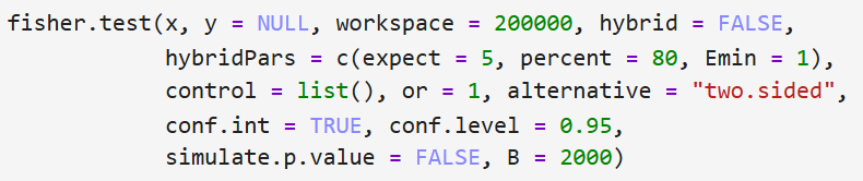
• x: This is a required parameter and represents the input data. It should be a contingency table, typically a matrix or a table with rows and columns representing categories or levels of two categorical variables. It is the observed data that you want to analyze using Fisher’s Exact Test.
• y: This parameter is optional. If you provide a second variable y, it should also be in a similar format as x. You can use this parameter when you want to perform a 2×2 Fisher’s Exact Test, and y represents the second variable’s data. If not provided, the function assumes a 2×2 contingency table with data in x.
• alternative: This parameter specifies the alternative hypothesis and controls the direction of the test. The options are:
  • “two.sided” (default): This is a two-tailed test where you’re interested in whether there’s an association between the variables (not equal to the expected value).
  • “greater”: This is a one-tailed test for the alternative that the association is greater than expected.
  • “less”: This is a one-tailed test for the alternative that the association is less than expected.
• conf.int: This is a logical parameter (TRUE or FALSE) that determines whether to compute a confidence interval for the odds ratio. If set to TRUE, the function will calculate a confidence interval; if set to FALSE, it won’t.

These are the key parameters for using the fisher.test function. Other parameters, such as workspace, hybrid, hybridPars, control, or, conf.level, simulate.p.value, B provide additional control and customization options for the Fisher’s Exact Test but are not essential for basic usage.

Synthetic datasets

Here, we will generate two datasets to practice using R for Fisher’s Exact Test.

2 x 2 Data

Here, we will create a synthetic dataset representing a contingency table often encountered in psychology research. In this example, we will consider a hypothetical study examining the relationship between two categorical variables: “Treatment” and “Outcome.”

# Create the dataset
set.seed(123) # for reproducibility

# Define levels for the variables
treatment_levels <- c("A", "B")
outcome_levels <- c("Improved", "Not Improved")

# Generate random data
n <- 200 # Total number of observations
treatment <- sample(treatment_levels, n, replace = TRUE)
outcome <- sample(outcome_levels, n, replace = TRUE)

# Create a dataframe
data_df <- data.frame(Treatment = treatment, Outcome = outcome)



# View the first few rows of the dataset
head(data_df)Code language: R (r)

In the code chunk above, we have generated a synthetic dataset tailored to mimic a scenario encountered in Psychology research. This dataset includes two categorical variables, “Treatment” and “Outcome,” with predefined levels representing different treatment groups and treatment outcomes. Here are the first few rows:

• Save

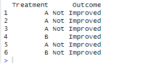
Next, we used the sample() function to generate random data for both variables. Then, we used the set.seed(123) command to ensure the reproducibility of the generated data. Subsequently, we combined the two variables into a data frame named “data_df.”

2 x 3 Data

Here is how we can generate data for a 2 x 3 contingency table:

# Load necessary libraries
library(dplyr)

# Create the dataset
set.seed(789) # for reproducibility

# Define levels for the variables
psychology_levels <- c("Anxiety", "Depression", "Stress")
hearing_levels <- c("Hearing Loss", "No Hearing Loss")

# Generate random data
n <- 300 # Total number of observations

# Create data to make Fisher's Exact Test significant
psych <- c(sample(c("Anxiety", "Depression"), n / 2, replace = TRUE),
                sample(c("Anxiety", "Depression", "Stress"), n / 2, replace = TRUE))
hearing <- c(rep("Hearing Loss", n / 2), rep("No Hearing Loss", n / 2))

# Shuffle the data randomly
shuffled_index <- sample(1:n)
psychology <- psych[shuffled_index]
hearing <- hearing[shuffled_index]

# Create a data frame
data_df2x3 <- data.frame(Psychology = psych , Hearing_Status = hearing)Code language: PHP (php)

In the code snippet above, we start the random data generation process while ensuring reproducibility using the set.seed(789) function.

To construct our dataset, we defined the possible levels for two categorical variables: Psychology and Hearing_Status. These variables represent psychological conditions, including “Anxiety,” “Depression,” and “Stress,” as well as hearing status, which can be either “Hearing Loss” or “No Hearing Loss.”

Then, we specified 300 observations, denoted as ‘n.’ This test assesses the relationship between two categorical variables.

We generated a Psychology variable with two distinct groups. The first half of the observations consist of “Anxiety” and “Depression,” while the second half introduces a broader set that includes “Stress.” The Hearing_Status variable is equally divided into “Hearing Loss” and “No Hearing Loss.”

Next, we used the ifelse() function combined with the %in% operator. It ensured that when the Psychology variable includes “Anxiety” or “Depression,” the Hearing_Status variable is more likely to be assigned “Hearing Loss” with a probability of 0.8, compared to “No Hearing Loss” with a probability of 0.2. Conversely, when the Psychology variable is “Stress,” the Hearing_Status variable is distributed equally between the two categories with a probability of 0.5 for each.

Then, we shuffled the data to introduce variability. This was achieved by creating a random permutation index using sample(1:n) and applying it to both the Psychology and Hearing_Status variables. Finally, we combined these variables into a cohesive dataframe named data_df3x2, which is now ready for further analysis

With these synthetic datasets, we can easily create a cross-tabulation (contingency table) in R to explore these relationships. In the following sections, we will use the datasets for practicing Fisher’s Exact Test and interpreting its results in the context of Psychology research.

Creating a Cross-Tabulation (Contingency Table) in R

Now that our synthetic data is ready, we can create a a cross-tabulation (contingency table) in R.

# Create a contingency table
contingency_table <- table(data_df$Treatment, data_df$Outcome)

# Display the contingency table
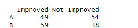
contingency_tableCode language: R (r)

In the code snippet above, we first defined a contingency table using the table() function, specifying the two categorical variables, Treatment and Outcome, from our synthetic data. The resulting table provides a clear view of how the categories are distributed within these variables, which is essential for further analysis, including the Fisher’s Exact Test we will perform in the next section.

• Save

Performing Fisher’s Exact Test in R

We can use the fisher.test() function to perform Fisher’s Exact Test in R.

# Perform Fisher's Exact Test
fisher_result <- fisher.test(contingency_table)

# Display the Fisher's Exact Test result
fisher_result
Code language: R (r)

In the code chunk above, we used the fisher.test() function on the contingency table to carry out Fisher’s Exact test in R. This test will help us assess whether there are significant associations between the two categorical variables, Treatment and Outcome.

• Save

How to Interpret Fisher’s Exact Test Results

Interpreting the results of Fisher’s Exact Test is crucial to draw meaningful conclusions from the analysis. Let us examine the output of the test to understand its components.

# Interpret the Fisher's Exact Test results
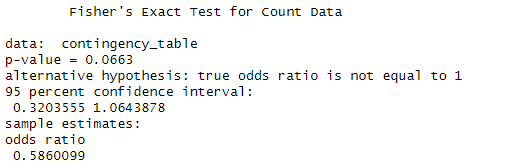
print(fisher_result)Code language: R (r)

In the code chunk above, printed the fisher_result object to obtain the statistics and p-values to help us make informed decisions based on the test’s outcome (i.e., enabling us to interpret the results). We can interpret the Fisher’s Exact test results we obtained using R as follows. First, the p-value equals 0.0663. This p-value indicates the statistical significance of the observed association between the variables. Remember, in the context of hypotheses testing, a p-value below a significance level (e.g., 0.05) indicates statistical significance. In this case, the p-value is higher than 0.05, suggesting that the association between the two categorical variables (Psychology and Hearing Status) is not statistically significant.

Odds Ratio

The estimated odds ratio is 0.586. Remember that the odds ratio represents the odds of one group (e.g., a specific psychological condition) compared to another group (e.g., hearing status). An odds ratio of less than 1 indicates a decreased odds or a potential negative association. However, the estimate is not significantly different from 1, as indicated by the confidence interval, reinforcing the notion that the association may not be substantial.

Post Hoc Analysis with Fisher’s Exact Test

After conducting Fisher’s Exact Test and obtaining significant results, we may want to explore further to understand which categories contribute to the significance. Post hoc analysis can be valuable in this regard. We will use the pairwise.fisher.test() function to perform pairwise comparisons between levels of the Treatment variable.

library(reporttools)
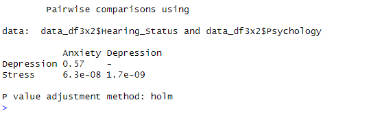
pairwise.fisher.test(data_df3x2$Hearing_Status, 
                                  data_df3x2$Psychology,
                                  p.adjust.method = "holm")Code language: R (r)

In the code chunk above, we learned how to conduct a post hoc analysis with Fisher’s Exact Test, focusing on pairwise comparisons between different levels of the Psychology variable. This additional analysis can provide deeper insights into the relationships between categories within our categorical variables.

• Save

Interpreting the Post Hoc Analysis

The results of the pairwise comparisons between “Hearing Status” and “Psychology” categories indicate the following:

1. Anxiety vs. Depression: The p-value for comparing “Anxiety” and “Depression” is 0.23. This p-value suggests no statistically significant difference in the distribution of these two categories concerning hearing status. In other words, individuals with anxiety and those with depression do not show a significant difference in their hearing status.
2. Depression vs. Stress: The p-value for comparing “Depression” and “Stress” is less than 2e-16. This p-value indicates a significant difference in the distribution of hearing status between individuals with depression and those with stress. In practical terms, it suggests that individuals with depression and those with stress have significantly different hearing status patterns.

The p-value adjustment method used here is “holm,” (e.g., Holm, 1978), one of several methods for correcting p-values in multiple comparisons to control the familywise error rate.

Plot Fisher’s Exact Test in R

We can use ggstatsplot to visualize the results:

library(ggstatsplot)
library(ggplot2)

fisher_results <- fisher.test(table(data_df3x2))

# Assuming your data frame is called 'data_df3x2'
# Replace "Psychology" and "Hearing_Status"
# with your actual variable names
# Also replace "fisher_results"
ggbarstats(
  data = data_df3x2,
  x = Psychology,
  y = Hearing_Status,
  results.subtitle = FALSE,
  subtitle = paste0(
    "Fisher's Exact Test", ", p-value ",
    ifelse(fisher_results$p.value < 0.001, 
           "< 0.001", paste("=", round(fisher_results$p.value, 3)))
  ),
  ggtheme = theme_bw()
) Code language: R (r)

In the code chunk above, we used the ggstatsplot and ggplot2 libraries to visualize the results from a Fisher’s Exact test in an easily interpretable manner. Initially, we used R to perform the Fisher’s Exact Test with the fisher.test() function on a contingency table created with table(data_df3x2).

• Save

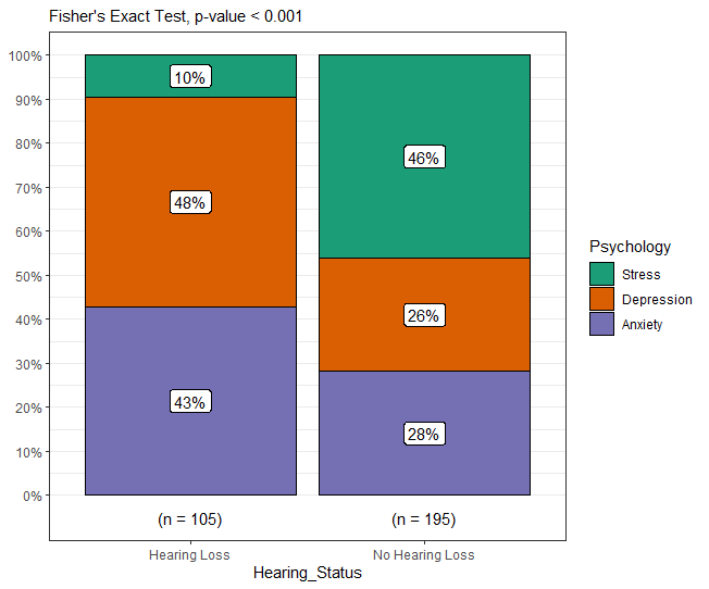
Subsequently, we used the ggbarstats() function to generate a grouped bar plot. The plot we generated visualizes the association between two categorical variables, Psychology and Hearing_Status, which should be replaced with your actual variable names. We also added a subtitle that provides key information, including the test conducted (Fisher’s Exact Test) and the associated p-value, which is rounded to three decimal places or indicated as “< 0.001” if it is less than that threshold. Finally, we used the theme_bw()function to get the rectangle surrounding the plot. Here are some more ggplot2 tutorials:

• Plot Prediction Interval in R using ggplot2
• How to Create a Violin plot in R with ggplot2 and Customize it
• ggplot Center Title: A Guide to Perfectly Aligned Titles in Your Plots
• Plot Prediction Interval in R using ggplot2
• How to Make a Scatter Plot in R with Ggplot2

Fisher’s Exact Test vs. Chi-Square Test

When dealing with categorical data and assessing associations between variables, we might wonder whether to use Fisher’s Exact Test or the Chi-Square Test. Both tests are valuable tools, but they have different applications and assumptions.

Fisher’s Exact Test

• Suitable for small sample sizes.
• It does not assume that the marginal totals (row and column totals) are fixed.
• It is ideal when dealing with rare events or when the Chi-Square Test assumptions are unmet.

Chi-Square Test:

• Typically used with larger sample sizes.
• Assumes that the marginal totals are fixed.
• It is more suitable when we have a larger dataset and do not encounter issues with rare events.

The choice between these tests depends on the dataset’s characteristics and whether the assumptions of the Chi-Square Test are met. Fisher’s Exact Test is preferred when dealing with small samples or when the Chi-Square Test assumptions are violated. It provides an exact p-value but may be computationally intensive for larger datasets. In contrast, the Chi-Square Test is efficient for larger samples but relies on the assumption of fixed marginal totals.

Remember to consider the nature of the data and the specific research question to determine which test is most appropriate for your analysis.

Conclusion

In this post, we have covered the ins and outs of Fisher’s Exact Test in R. We began by establishing the prerequisites, ensuring you have a solid foundation. Then, we dived deep into Fisher’s Exact Test, unraveling its assumptions, hypotheses, and how to interpret its results.

You have learned how to perform Fisher’s Exact Test in R, allowing you to apply this statistical method to real-world datasets. The inclusion of synthetic datasets allowed for hands-on practice, reinforcing your understanding of the test’s mechanics. Additionally, we explored visualizing Fisher’s Exact Test results, providing you with effective tools for conveying your findings.

Finally, we compared Fisher’s Exact Test to the Chi-Square Test, offering insights into when to choose one over the other.
Please share your insights, experiences, and questions in the comments below. If you liked the post, share it on your social media accounts as well.

Frequently Asked Questions (FAQ)

References

Holm, S. (1979). A simple sequentially rejective multiple test procedure. Scandinavian journal of statistics, 65-70.

Additional Resources

Here are some more great tutorials on this site:

• How to Rename Column (or Columns) in R with dplyr
• Cronbach’s Alpha in R: How to Assess Internal Consistency
• How to Sum Rows in R: Master Summing Specific Rows with dplyr
• Correlation in R: Coefficients, Visualizations, & Matrix Analysis
• How to Create a Sankey Plot in R: 4 Methods
• Countif function in R with Base and dplyr
• Coefficient of Variation in R