Cronbach’s Alpha in R: How to Assess Internal Consistency

In this tutorial, we will learn how to calculate Cronbach’s alpha in R, a measure for assessing the internal consistency of a set of related variables. Internal consistency indicates the reliability of a scale or instrument used to measure a particular construct, such as psychological traits or survey responses. Cronbach’s alpha can provide insights into how well the items within a scale are correlated with each other, offering a glimpse into the overall reliability of the measurements.

Ensuring their internal consistency is crucial for valid and reliable data analysis when dealing with multiple-item scales or questionnaires. We will explore how to calculate Cronbach’s alpha using R.

• Save

This tutorial will focus on Cronbach’s alpha and its significance, particularly in psychology, where reliable measurements are crucial for drawing meaningful conclusions from research studies and surveys.

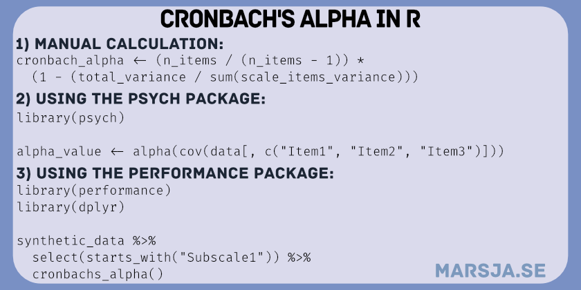
Table of Contents

• Outline
• Prerequisites
• Cronbach’s Alpha:
  • Calculating Cronbach’s Alpha:
  • Interpreting Cronbach’s Alpha:
• Example: Internal Consistency in Hearing Science
• Synthetic Data
  • Exploring the Data
• Manually Calculating Cronbach’s Alpha in R with dplyr
  • Step 1: Calculate Variance per Item
  • Step 2: Calculate Total Variance
  • Step 3: Calculate Cronbach’s Alpha
  • Calculating Cronbach’s Alpha for a Subscale
• Cronbach’s Alpha using the R package psych
• Calculating Cronbach’s Alpha in R with the performance Package
• Conclusion
• Summary
• Resources

Outline

The structure of the post is as follows: We begin by providing the necessary prerequisites for following this post. We then get into the topic’s core, covering its calculation step by step using manual methods and R packages. We explore how to interpret the calculated alpha values and showcase their application using an example from hearing science. The post also introduces synthetic data and walks through data exploration techniques. We examine different approaches for calculating alpha, including manual calculations, using the psych package, and utilizing the performance package. The post culminates with a concise conclusion summarizing the key takeaways and inviting you to share your insights and experiences.

Prerequisites

Before we learn how to get Cronbach’s Alpha in R, it is essential to establish a solid foundation. Here is what you need to have in place:

First, a fundamental understanding of internal consistency and psychometric measurement concepts is crucial. This includes comprehending the significance of Cronbach’s Alpha as a measure of reliability and interpreting its values accurately.

Furthermore, a basic familiarity with R programming is necessary. Suppose you are comfortable with concepts like data frames, functions, and manipulation using packages like dplyr and tidyr. In that case, you will be better equipped to follow along and implement the techniques demonstrated.

You will need a few essential R packages to execute the examples in this post. The tidyverse suite, encompassing popular packages such as dplyr and tidyr plays an important role. dplyr aids in efficient data manipulation, tidyr enables data tidying and reshaping

We will also use the psych package to perform psychometric calculations, including Cronbach’s Alpha. To ensure you have these packages installed, use the install.packages() function in R:

install.packages(c('dplyr', 'MASS', 'tibble', 'performance'))Code language: JavaScript (javascript)

Remember to update your R version to access the latest features and improvements by executing installr::updateR(). To verify your R version, use the command R.version$version.string within the R console.

As previously mentioned, this post will show the power of the dplyr package, which can be used for more than Cronbach’s Alpha calculation. The dplyr packages enable you to perform many data manipulation tasks effortlessly. From using dplyr’s select() to remove specific columns and identify duplicate rows to conducting count operations and data summarization, dplyr proves invaluable for enhancing your data analysis capabilities.

Cronbach’s Alpha:

Cronbach’s alpha, often called coefficient alpha, is a widely used measure of internal consistency reliability. It assesses how well a set of items within a scale or questionnaire correlates, providing insight into the extent to which the items measure a common underlying construct. Higher alpha values indicate greater internal consistency and reliability.

Calculating Cronbach’s Alpha:

We need the individual responses for each item in the scale to calculate Cronbach’s alpha. The formula involves summing up all items’ variances and the total score’s variance, then dividing the former by the latter. The alpha() function from the “psych” package simplifies this process in R.

Interpreting Cronbach’s Alpha:

Cronbach’s alpha ranges between 0 and 1, with higher values indicating better internal consistency. However, no fixed threshold exists for an “acceptable” alpha value—it depends on the context and field of study. Generally, an alpha above 0.7 is considered adequate, while values above 0.8 are preferred for more precise measurements.

Example: Internal Consistency in Hearing Science

Consider the Speech, Spatial, and Qualities scale (SSQ), a tool used to assess auditory perception and spatial hearing abilities in individuals with hearing impairments. The SSQ comprises various items related to speech understanding, sound localization, and quality of sound perception. Ensuring internal consistency in the SSQ is vital to ensure that the items consistently measure the intended auditory constructs. By calculating Cronbach’s alpha for the SSQ items, we can determine whether the scale is reliable for evaluating the different dimensions of auditory perception in individuals with hearing difficulties. This analysis aids researchers and clinicians in making accurate and informed conclusions about hearing-related outcomes.

In the following sections, we will dive into hands-on examples of calculating Cronbach’s alpha in R, providing you with the skills to check the internal consistency of your data. First, however, we will generate a synthetic dataset that you can use to practice.

Synthetic Data

Here, we generate synthetic data to practice using R to calculate Cronbach’s alpha:

library(MASS)       # For mvrnorm()
library(dplyr)
library(tibble)

set.seed(20230826)

# Generate participant IDs
participant_id <- seq(1, 100)

# Create a correlation matrix for the items
correlation_matrix <- matrix(c(
  1, 0.61, 0.62, 0.21, 0.23, 0.21, 0.24, 0.27, 0.21,
  0.64, 1, 0.61, 0.23, 0.21, 0.21, 0.22, 0.23, 0.24,
  0.61, 0.7, 1, 0.23, 0.71, 0.29, 0.23, 0.21, 0.23,
  0.26, 0.28, 0.21, 1, 0.63, 0.58, 0.26, 0.22, 0.23,
  0.21, 0.23, 0.24, 0.67, 1, 0.61, 0.27, 0.26, 0.28,
  0.23, 0.24, 0.26, 0.66, 0.63, 1, 0.25, 0.26, 0.24,
  0.28, 0.27, 0.26, 0.25, 0.24, 0.23, 1, 0.63, 0.64,
  0.21, 0.23, 0.23, 0.24, 0.26, 0.23, 0.55, 1, 0.61,
  0.27, 0.26, 0.25, 0.24, 0.26, 0.21, 0.63, 0.7, 1
), ncol = 9, byrow = TRUE)

# Generate correlated data
correlated_data <- mvrnorm(n = 100, mu = rep(4, 9),
                           Sigma = correlation_matrix)

# Create a tibble from the synthetic data
synthetic_data <- as_tibble(correlated_data)

# Rename columns
colnames(synthetic_data) <- c(
  "Subscale1_Item1", "Subscale1_Item2", "Subscale1_Item3",
  "Subscale2_Item1", "Subscale2_Item2", "Subscale2_Item3",
  "Subscale3_Item1", "Subscale3_Item2", "Subscale3_Item3"
)Code language: R (r)

In the code snippet above, we first loaded the necessary libraries, including the MASS library for the mvrnorm() function and the dplyr and tibble libraries. To ensure reproducibility, we set a seed value using set.seed(). We then created a sequence of numbers using the seq() function. These participant IDs range from 1 to 100.

We construct a matrix in R that defines relationships among the different items in our synthetic data. This matrix reflects how each item within and across subscales is correlated. The values in this matrix range from 0.21 to 1, with correlations within the same subscale being higher, aiming for a range of 0.5 to 0.7, while correlations between different subscales are lower, usually below 0.3.

Subsequently, we generate synthetic data using the mvrnorm() function, which simulates multivariate normal distributions based on the correlation matrix. The mu argument defines the means for each subscale, set here to a common value of 4.

We then convert the generated data into a tibble using the as_tibble() function. The column names are assigned to each item of the subscales. This structured data format allows for better organization and analysis.

In the next step, we will create a correlation matrix of the data and visualize it for a quick overview.

Exploring the Data

Here we have a quick look at the synthetic data:

library(ggcorrplot)

# Create a correlation plot
correlation_matrix <- cor(synthetic_data)
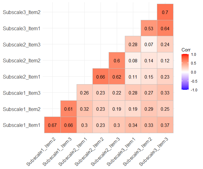
ggcorrplot(correlation_matrix, type = "lower", lab = TRUE)Code language: R (r)

In the code chunk above, we created a correlation matrix using R’s cor() function, which calculates the pairwise correlations between variables in the synthetic data. This matrix captures the strength and direction of relationships between the different subscale items. We then employed the ggcorrplot package to generate a correlation plot. Here, we can see that there are higher correlations between items within a subscale than between:

• Save

In the next section, we will learn how to manually calculate Cronbach’s alpha with the R package dplyr.

Manually Calculating Cronbach’s Alpha in R with dplyr

To calculate Cronbach’s alpha for the entire questionnaire using R and the dplyr package, we can use the following three steps:

Step 1: Calculate Variance per Item

In this step, we start by calculating the mean score for each item across all participants in the dataset.

library(dplyr)

item_means <- synthetic_data %>%
  summarise_all(mean)

squared_diff <- synthetic_data %>%
  mutate(across(everything(), ~ (. - item_means[[cur_column()]])^2))

sum_squared_diff <- squared_diff %>%
  summarise(across(everything(), sum))

n_participants <- nrow(subscale_items)
scale_variance <- sum_squared_diff / (n_participants - 1)Code language: R (r)

In the code snippet above, we used the dplyr package to perform a series of calculations to evaluate the internal consistency of the questionnaire items.

We used the %>% pipe operator and the summarise_all(mean) function to calculate the mean score for each item in the dataset. This step creates a summary of the item means.

Next, we combined the mutate() function with the across() function to compute the squared differences between each participant’s score and the mean score for every item.

Subsequently, we progress to determine the sum of squared differences for each item across all participants. To achieve this, we again used the %>% operator, followed by the summarise() function with across(everything(), sum) applied.

We compute the total number of participants, n_participants, using the nrow() function on the subscale_items dataset.

Lastly, we calculated scale_variance by dividing the previously computed sum of squared differences by the number of participants minus one (n-1).

Step 2: Calculate Total Variance

The second step involves summing up the variances calculated in Step 1 for all items. Total variance is an overall measure of variability within the questionnaire:

total_variance <- sum(scale_variance)Code language: R (r)

In the code block above, we calculated the total variance using the sum() function on the variance of the subscales.

Step 3: Calculate Cronbach’s Alpha

In the final step, we calculate Cronbach’s alpha using the formula:

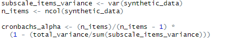
scale_items_variance <- var(synthetic_data)
n_items <- ncol(synthetic_data)
cronbach_alpha <- (n_items / (n_items - 1)) * 
  (1 - (total_variance / sum(scale_items_variance)))Code language: R (r)

In the code chunk above, we calculate essential components to derive Cronbach’s Alpha, a measure of internal consistency. Firstly, we computed the subscale_items_variance using the var() function.

Next, we determined the total number of items within the subscale using the ncol() function. Remember, if there are other variables in your dataset, only select the columns you need (i.e., the items).

Here, we applied the determined values of n_items, total_variance, and subscale_items_variance to compute Cronbach’s Alpha.

Calculating Cronbach’s Alpha for a Subscale

We can adapt the earlier process to assess the internal consistency of individual subscales within a questionnaire. In the following code example, we will use dplyr to select columns by their name (the items). This way, we can compute Cronbach’s alpha for each subscale individually.

subscale_data <- synthetic_data %>%
  select(Subscale1_Item1:Subscale1_Item3)  # Replace with appropriate column names
Code language: R (r)

Next, we can apply the same procedure to calculate the variance, total variance, and Cronbach’s alpha for the selected subscale. We use the same code as the previous example but on the subsetted data (i.e., the items we selected).

subscale_item_means <- subscale_data %>%
  summarise_all(mean)

subscale_squared_diff <- subscale_data %>%
  mutate(across(everything(), ~ (. - subscale_item_means[[cur_column()]])^2))

subscale_sum_squared_diff <- subscale_squared_diff %>%
  summarise(across(everything(), sum))

subscale_variance <- subscale_sum_squared_diff / (n_subscale_items - 1)

total_variance <- sum(subscale_variance)

subscale_items_variance <- var(subscale_data)
cronbach_alpha_subscale <- (n_subscale_items / (n_subscale_items - 1)) * 
  (1 - (total_variance / sum(subscale_items_variance)))Code language: R (r)

Additionally, we can calculate Cronbach’s alpha for all subscales using the lapply() function and a custom function when we have multiple subscales. This approach streamlines the process further and provides alpha values for each subscale more efficiently.

library(dplyr)

calculate_alpha <- function(data, items) {
  item_means <- data %>%
    select(all_of(items)) %>%
    summarise_all(mean)
  
  item_variances <- data %>%
    select(all_of(items)) %>%
    summarise_all(var)
  
  total_variance <- sum(item_variances)
  scale_variance <- var(rowSums(select(data, all_of(items))))
  
  alpha <- (length(items) / (length(items) - 1)) * (1 - (total_variance / scale_variance))
  return(alpha)
}

subscales <- list(
  c("Subscale1_Item1", "Subscale1_Item2", "Subscale1_Item3"),
  c("Subscale2_Item1", "Subscale2_Item2", "Subscale2_Item3"),
  c("Subscale3_Item1", "Subscale3_Item2", "Subscale3_Item3")
)

alpha_results <- unlist(lapply(subscales, calculate_alpha, data = synthetic_data))

result_df <- tibble(Subscale = c("Subscale1", "Subscale2", "Subscale3"),
                    Cronbachs_Alpha = alpha_results)
print(result_df)Code language: PHP (php)

In the code chunk above, we created a custom function called calculate_alpha. This function streamlines the process of calculating Cronbach’s alpha for subscales. The function takes two inputs: the dataset (data) and a character vector of subscale item names (items). It then computes alpha using the variances of the subscale items and the row sums.

Next, we defined the subscale items for which we want to calculate Cronbach’s alpha. We organize these items into a list named subscales. Each list element is a vector containing the column names of the items within a subscale.

We then used the lapply() function to apply the custom function to each subscale in the subscales list. The data argument is set to our synthetic_data dataset. The result is a list of alpha values, one for each subscale. We use the unlist() function to convert the Cronbach’s Alpha results list into a vector.

To summarize and display the calculated alpha values, we created a tibble named result_df. This table comprises two columns: “Subscale” to identify each subscale and “Cronbachs_Alpha” to show the corresponding alpha value.

As previously mentioned, alternative methods are available in R to calculate Cronbach’s alpha using the psych and performance packages. While these approaches are convenient, they require the packages to be installed and updated. Let us explore how to use these packages to calculate alpha.

Cronbach’s Alpha using the R package psych

We can use the alpha() function from the psych package to calculate alpha for a subscale.

library(psych)

alpha_value <- alpha(cov(synthetic_data[, c("Subscale1_Item1", "Subscale1_Item2", "Subscale1_Item3")]))Code language: CSS (css)

In the code chunk above, we first use the alpha() function from the psych package to calculate Cronbach’s alpha for a subscale. This function requires a covariance matrix as input, which can be obtained using the cov() function. The subscale items are selected from the synthetic_data using column indexing.

• Save

This code snippet is another way to use R to calculate Cronbach’s alpha for a specific subscale. We do this by utilizing the psych package’s alpha() function, and it allows us to assess the internal consistency and reliability of the subscale’s items based on their covariance matrix. Note that we need to run the code for each subscale.

Calculating Cronbach’s Alpha in R with the performance Package

Here is another approach to calculating Cronbach’s alpha using the performance package in R:

library(performance)
library(dplyr)

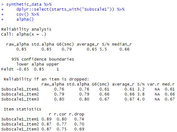
synthetic_data %>% 
  select(starts_with("Subscale1")) %>%
  cronbachs_alpha() Code language: JavaScript (javascript)

In the code chunk above, we used the select() function from the dplyr package to choose all columns that start with “Subscale1” from the synthetic_data dataframe. These selected columns represent the items belonging to the “Subscale1” subscale. We then applied the cronbachs_alpha() function from the performance package to calculate Cronbach’s alpha for this subscale. We can repeat the code and change it to “Subscle2” to calculate internal consistency for the second subscale.

• Save

Conclusion

In this post about calculating Cronbach’s alpha in R, we explored multiple methods, each with advantages and considerations. As demonstrated earlier, manually computing Cronbach’s alpha provides a deeper understanding of the underlying calculations and reduces reliance on external packages, potentially ensuring stability over time.

• Save

However, this approach requires meticulous implementation, making it more susceptible to human error and less time-efficient for larger datasets. On the other hand, the psych package offers a comprehensive suite of functions for psychometric analysis, including Cronbach’s alpha. While relying on packages like psych and performance provides convenience and reliability, it introduces a dependency on the maintenance and updates of these packages in the future. For instance, the performance package’s specialization in checking assumptions and conducting robust statistical evaluations complements its Cronbach’s alpha calculation functionality.
Furthermore, leveraging the power of dplyr and tibble with these packages streamlines data manipulation. In summary, choosing the most suitable method depends on factors such as the complexity of the analysis, reliance on specific packages, and familiarity with manual calculations. Each approach has its place in the toolkit of a data analyst, offering a balance between insight, efficiency, and reliance on external libraries.

Summary

In this post, we have explored the calculation of Cronbach’s alpha, a measure for assessing internal consistency in scales and questionnaires. Starting with an introduction to its significance, we learned step-by-step procedures to calculate Cronbach’s alpha manually using R’s dplyr package. We looked at how to determine variance per item, total variance, and ultimately Cronbach’s alpha, accompanied by an example from hearing science. Demonstrating further versatility, we introduced a method for calculating Cronbach’s alpha for specific subscales, enhancing the applicability. Additionally, we explored alternatives, employing the psych and performance packages for automated alpha calculations.

Please share your thoughts and preferences in the comments below. Which method resonated with you the most, and how do you envision implementing Cronbach’s alpha in your data analysis? Feel free to discuss and share this post with colleagues. It is highly appreciated.

Resources

• Coefficient of Variation in R
• Probit Regression in R: Interpretation & Examples
• Cross-Tabulation in R: Creating & Interpreting Contingency Tables
• How to Create a Sankey Plot in R: 4 Methods
• How to Standardize Data in R
• How to Sum Rows in R: Master Summing Specific Rows with dplyr