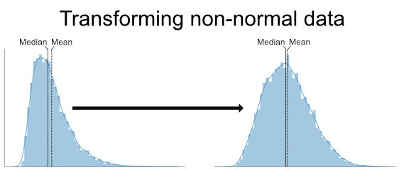
How to use Square Root, log, & Box-Cox Transformation in Python

In this tutorial, related to data analysis in Python, you will learn how to deal with your data when it is not following the normal distribution. One way to deal with non-normal data is to transform your data. In this post, you will learn how to carry out Box-Cox, square root, and log transformation in Python.

Transforming skewed data in Python — Transforming right skewed data to normal distribution

That the data we have is of normal shape (also known as following a Bell curve) is important for the majority of the parametric tests we may want to perform. This includes regression analysis, the two-sample t-test, and Analysis of Variance that can be carried out in Python, to name a few.

Outline
Prerequisites
Skewness and Kurtosis
Transformation Methods
Example Data
Visually Inspect the Distribution of Your Variables
Measures of Skewness and Kurtosis in Python
Square Root Transformation in Python
- Transforming Negatively Skewed Data with the Square Root Method
Log Transformation in Python
- Log Transforming Negatively Skewed Data
Box-Cox Transformation in Python
Conclusion
References

Outline

This post will start by briefly reviewing what you need to follow this tutorial. After this is done, you will 1) get information about skewness and kurtosis, and 2) a brief overview of the different transformation methods. In the section following the transformation methods, you will learn how to import data using Pandas read_csv. We will explore the example dataset a bit by creating histograms, and getting the measures of skewness and kurtosis. Finally, the last sections will cover how to transform data that is non-normal.

Prerequisites

In this tutorial, we are going to use Pandas, SciPy, and NumPy. It is worth mentioning, here, that you only need to install Pandas as the other two Python packages are dependencies of Pandas. That is, if you install Python packages using e.g. pip it will also install SciPy and NumPy on your computer, whether you use e.g. Ubuntu Linux or Windows 10. Note, that you can use pip to install a specific version of e.g. Pandas and if you need, you can upgrade pip using either conda or pip.

Now, if you want to install the individual packages (e.g. you only want to use NumPy and SciPy) you can run the following code:

pip install pandasCode language: Bash (bash)

Now, if you only want to install NumPy, change “pandas” to “numpy”, in the code chuk above. That said, let us move on to the section about skewness and kurtosis.

Skewness and Kurtosis

Briefly, skewness is a measure of symmetry. To be exact, it is a measure of lack of symmetry. This means that the larger the number is the more your data lack symmetry (not normal, that is). Kurtosis, on the other hand, is a measure of whether your data is heavy- or light-tailed relative to a normal distribution. See here for a more mathematical definition of both measures. A good way to visually examine data for skewness or kurtosis is to use a histogram. Note, however, that there are, of course, also different statistical tests that can be used to test if your data is normally distributed.

How do you handle skewed data in Python?

One way to handle right or left skewed data is to carry out the logarithmic transformation on our data. For example, np.log(x) will log transform the variable x in Python. There are other options and the Box-Cox and Square root transformations.

How do you convert left skewed data?

One way to handle left (negative) skewed data is to reverse the distribution of the variable. In Python, this can be done using the following code:

Both of the above questions will be more detailed and answered throughout the post (e.g., you will learn how to carry out log transformation in Python). In the next section, you will learn about the three commonly used transformation techniques that you will also learn to apply later.

Transformation Methods

As indicated in the introduction, we are going to learn three methods that we can use to transform data deviating from the normal distribution. In this section, you will get a brief overview of these three transformation techniques and when to use them.

Square Root

The square root method is typically used when your data is moderately skewed. Now using the square root (e.g., sqrt(x)) is a transformation that moderately affects the distribution shape. It is generally used to reduce right-skewed data. Finally, the square root can be applied to zero values and is most commonly used on counted data.

Log Transformation

The logarithmic is a strong transformation that has a major effect on distribution shape. This technique is, as the square root method, often used for reducing right skewness. Worth noting, however, is that it can not be applied to zero or negative values.

Box-Cox Transformation

The Box-Cox transformation is, as you probably understand, also a technique to transform non-normal data into normal shape. This is a procedure to identify a suitable exponent (Lambda = l) to use to transform skewed data.

Other Alternatives

Now, the above mentioned transformation techniques are the most commonly used. However, there are plenty of other methods, as well, that can be used to transform your skewed dependent variables. For example, if your data is of ordinal data type you can also use the arcsine transformation method. Another method that you can use is called reciprocal. This method is basically carried out like this: 1/x, where x is your dependent variable.

In the next section, we will import data containing four dependent variables that are positively and negatively skewed.

Example Data

In this tutorial, we will transform data that is both negatively (left) and positively (right) skewed and we will read an example dataset from a CSV file (Data_to_Transform.csv). To our help, we will use Pandas to read the .csv file:

import pandas as pd
import numpy as np

# Reading dataset with skewed distributions
df = pd.read_csv('./SimData/Data_to_Transform.csv')Code language: Python (python)

This is an example dataset that has the following four variables:

Moderate Positive Skew (Right Skewed)
Highly Positive Skew’ (Right Skewed)
Moderate Negative Skew (Left Skewed)
Highly Negative Skew (Left Skewed)

We can obtain this information by using the info() method. This will give us the structure of the dataframe:

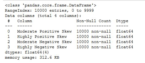
Structure of Pandas dataframe containing 4 skewed data to transform to normal distribution.

As you can see, the dataframe has 10000 rows and 4 columns (as previously described). Furthermore, we get the information that the 4 columns are of float data type and that there are no missing values in the dataset. In the next section, we will have a quick look at the distribution of our 4 variables.

In the next section, we will do a quick visual inspection of the variables in the dataset using Pandas hist() function.

Visually Inspect the Distribution of Your Variables

In this section, we are going to visually inspect whether the data are normally distributed. Of course, there are several ways to plot the distribution of our data. In this post, however, we are going to only use Pandas and create histograms. Here’s how to create a histogram in Pandas using the hist() method:

df.hist(grid=False,
       figsize=(10, 6),
       bins=30)Code language: Python (python)

Now, the hist() method takes all our numeric variables in the dataset (i.e.,in our case float data type) and creates a histogram for each. Just to quickly explain the parameters used in the code chunk above. First, using the grid parameter and set it to False to remove the grid from the histogram. Second, we changed the figure size using the figsize parameter. Finally, we also changed the number of bins (default is 20) to get a better view of the data. Here is the distribution visualized:

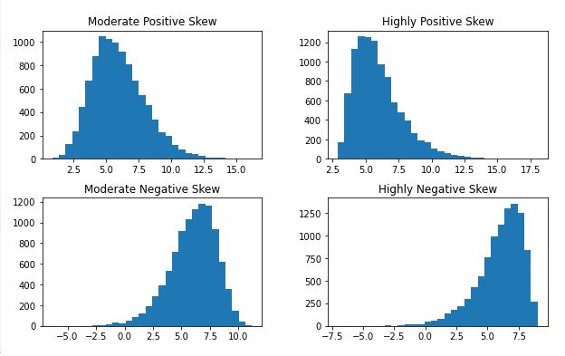
Pandas histogram showing skewness - right, and left, high and moderate — Histogram showing right and left skewed variables.

It is pretty clear that all the variables are skewed and not following a normal distribution (as the variable names imply). Note there are, of course, other visualization techniques that you can carry out to examine the distribution of your dependent variables. For example, you can use boxplots, stripplots, swarmplots, kernel density estimation, or violin plots. These plots give you a lot of (more) information about your dependent variables. See the post with 9 Python data visualization examples, for more information. In the next section, we will also look at how we can get the measures of skewness and kurtosis.

Measures of Skewness and Kurtosis in Python

In this section, before we start learning how to transform skewed data in Python, we will just have a quick look at how to get skewness and kurtosis in Python.

df.agg(['skew', 'kurtosis']).transpose()Code language: Python (python)

In the code chunk above, we used the agg() method and used a list as the only parameter. This list contained the two methods we wanted to use (i.e., we wanted to calculate skewness and kurtosis). Finally, we used the transpose() method to change the rows to columns (i.e., transpose the Pandas dataframe) to get an output that is a bit easier to check. Here’s the resulting table:

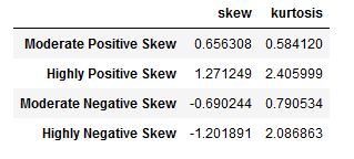
Skewness and kurtosis of dependent variables

As a rule of thumb, skewness can be interpreted like this:

	Skewness
Fairly Symmetrical	-0.5 to 0.5
Moderate Skewed	-0.5 to -1.0 and 0.5 to 1.0
Highly Skewed	< -1.0 and > 1.0

There are, of course, more things that can be done to test whether our data is normally distributed. For example, we can carry out statistical tests of normality, such as the Shapiro-Wilks test. However, it is worth noting that most of these tests are susceptible to the sample size. That is, even minor deviations from normality will be found using, e.g., the Shapiro-Wilks test.

In the next section, we will transform the non-normal (skewed) data. First, we will transform the moderately skewed distributions and then we will continue with the highly skewed data. Alternatives to transforming data:

Wilcoxon Signed-Rank test in Python

Square Root Transformation in Python

Here’s how to do the square root transformation of non-normal data in Python:

# Python Square root transformation
df.insert(len(df.columns), 'A_Sqrt',
         np.sqrt(df.iloc[:,0]))Code language: Python (python)

In the code chunk above, we created a new column/variable in the Pandas dataframe by using the insert() method. It is, furthermore, worth mentioning that we used the iloc[] method to select the column we wanted. In the following examples, we will continue using this method for selecting columns. Notice how the first parameter (i.e., “:”) is used to select all rows, and the second parameter (“0”) is used to select the first columns. If we, on the other hand, used the loc method, we could have selected by the column name. Here’s a histogram of our new column/variable:

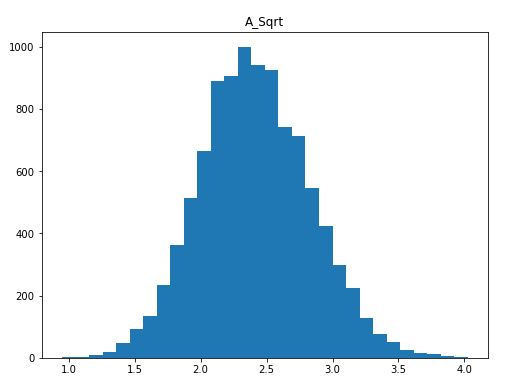
Again, we can see that the new, Box-Cox transformed, distribution is more symmetrical than the previous, right-skewed, distribution.

In the next subsection, you will learn how to deal with negatively (left) skewed data. If we try to apply sqrt() on the column, right now, we will get a ValueError (see towards the end of the post).

Transforming Negatively Skewed Data with the Square Root Method

Now, if we want to transform the negatively (left) skewed data using the square root method we can do as follows.

# Square root transormation on left skewed data in Python:
df.insert(len(df.columns), 'B_Sqrt',
         np.sqrt(max(df.iloc[:, 2]+1) - df.iloc[:, 2]))Code language: PHP (php)

What we did, above, was to reverse the distribution (i.e., max(df.iloc[:, 2] + 1) - df.iloc[:, 2]) and then applied the square root transformation. You can see, in the image below, that skewness becomes positive when reverting the negatively skewed distribution.

In the next section, you will learn how to log transform in Python on highly skewed data, both to the right and left.

Log Transformation in Python

Here’s how we can use the log transformation in Python to get our skewed data more symmetrical:

# Python log transform
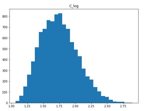
df.insert(len(df.columns), 'C_log',
         np.log(df['Highly Positive Skew']))Code language: PHP (php)

We did pretty much the same as when using Python to do the square root transformation. Here, we created a new column, using the insert() method. However, we used the log() method from NumPy, this time, because we wanted to do a logarithmic transformation. Here’s how the distribution looks like now:

Python log transformed distribution — Dependent Variable log Transformed in Python

Log Transforming Negatively Skewed Data

Here’s how to log transform negatively skewed data in Python:

# Log transformation of negatively (left) skewed data in Python
df.insert(len(df.columns), 'D_log',
         np.log(max(df.iloc[:, 2] + 1) - df.iloc[:, 2]))Code language: PHP (php)

Again, we transformed the log using the NumPy log() method. Furthermore, we did exactly as in the square root example. That is, we reversed the distribution and we can, again, see that all that happened is that the skewness went from negative to positive.

In the next section, we will have a look on how to use SciPy to carry out the Box Cox transformation on our data.

Box-Cox Transformation in Python

Here’s how to implement the Box-Cox transformation using the Python package SciPy:

from scipy.stats import boxcox

# Box-Cox Transformation in Python
df.insert(len(df.columns), 'A_Boxcox', 
              boxcox(df.iloc[:, 0])[0])Code language: Python (python)

In the code chunk above, the only difference, basically, between the previous examples is that we imported boxcox() from scipy.stats. Furthermore, we used the boxcox() method to apply the Box-Cox transformation. Notice how we selected the first element using the brackets (i.e. [0]). This is because this method (i.e. boxcox()) will give us a tuple. Here’s a visualization of the resulting distribution.

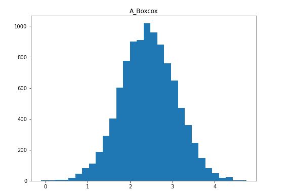
Histogram showing box-cox transformed data — Histogram of box-cox transformed dependent variable

Once again, we managed to transform our positively skewed data to a relatively symmetrical distribution. Now, the Box-Cox transformation also requires our data to only contain positive numbers so if we want to apply it to negatively skewed data we need to reverse it (see the previous examples on how to reverse your distribution). If we try to use boxcox() on the column “Moderate Negative Skewed”, for example, we get a ValueError.

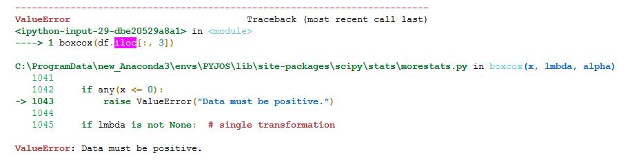
Trying to transforme negatively skewed data

More exactly, if you get the “ValueError: Data must be positive” while using either np.sqrt(), np.log() or SciPy’s boxcox() it is because your dependent variable contains negative numbers. To solve this, you can reverse the distribution.

It is worth noting, here, that we can now check the skewness using the skew() method:

df.agg(['skew']).transpose()Code language: Python (python)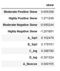

All variables transformed using the log, square root, and, box-cox methods in Python

We can see in the output that the skewness values of the transformed values are now acceptable (they are all under 0.5). Of course, we could also run the previously mentioned normality tests (e.g., the Shapiro-Wilks test). Note, that if your data is still not normally distributed, you can carry out the Mann-Whitney U test in Python, as well.

Conclusion

In this post, you have learned how to apply square root, logarithmic, and Box-Cox transformation in Python using Pandas, SciPy, and NumPy. Specifically, you have learned how to transform both positive (left) and negative (right) skewed data to hold the assumption of normal assumption. First, you learned briefly above the Python packages needed to transform non-normal and skewed data into normally distributed data. Second, you learned about the three methods that you later also learned how to carry out in Python.

References

Here are some useful resources for further reading.

DeCarlo, L. T. (1997). On the meaning and use of kurtosis. Psychological Methods, 2(3), 292–307. https://doi.org/10.1037//1082-989x.2.3.292

Blanca, M. J., Arnau, J., López-Montiel, D., Bono, R., & Bendayan, R. (2013). Skewness and kurtosis in real data samples. Methodology: European Journal of Research Methods for the Behavioral and Social Sciences, 9(2), 78–84. https://doi.org/10.1027/1614-2241/a000057

Mishra, P., Pandey, C. M., Singh, U., Gupta, A., Sahu, C., & Keshri, A. (2019). Descriptive statistics and normality tests for statistical data. Annals of cardiac anaesthesia, 22(1), 67–72. https://doi.org/10.4103/aca.ACA_157_18