In this Python data analysis tutorial, you will learn how to perform a paired sample t-test in Python. First, you will learn about this type of t-test (e.g. when to use it, the assumptions of the test). Second, you will learn how to check whether your data follow the assumptions and what you can do if your data violates some of the assumptions.
Third, you will learn how to perform a paired sample t-test using the following Python packages:
- Scipy (scipy.stats.ttest_ind)
- Pingouin (pingouin.ttest)
In the final sections, of this tutorial, you will also learn how to:
- Interpret and report the paired t-test
- P-value, effect size
- report the results and visualizing the data
In the first section, you will learn about what is required to follow this post.
Prerequisites
In this tutorial, we are going to use both SciPy and Pingouin, two great Python packages, to carry out the dependent sample t-test. Furthermore, to read the dataset we are going to use Pandas. Finally, we are also going to use Seaborn to visualize the data. In the next three subsections, you will find a brief description of each of these packages.
SciPy
SciPy is one of the essential data science packages. This package is, furthermore, a dependency of all the other packages that we are going to use in this tutorial. In this tutorial, we are going to use it to test the assumption of normality as well as carry out the paired sample t-test. This means, of course, that if you are going to carry out the data analysis using Pingouin you will get SciPy installed anyway.
Pandas
Pandas is also a very great Python package for someone carrying out data analysis with Python, whether a data scientist or a psychologist. In this post, we will use Pandas import data into a dataframe and to calculate summary statistics.
Seaborn
In this tutorial, we are going to use data visualization to guide our interpretation of the paired sample t-test. Seaborn is a great package for carrying out data visualization (see for example these 9 examples of how to use Seaborn for data visualization in Python).
Pingouin
In this tutorial, Pingouin is the second package we will use to do a paired sample t-test in Python. One great thing with the ttest function is that it returns a lot of information we need when reporting the results from the test. For instance, when using Pingouin we also get the degrees of freedom, Bayes Factor, power, effect size (Cohen’s d), and confidence interval.
How to Install the Needed Packages
In Python, we can install packages with pip. To install all the required packages, run the following code:
pip install scipy pandas seaborn pingouinCode language: Bash (bash)Note if you get a notification that there is a newer version available for Pip: you can easily upgrade pip from the command line. In the next section, we are going to learn about the paired t-test and the assumptions of the test.
Paired Sample T-test
The paired sample t-test is also known as the dependent sample t-test, and paired t-test. Furthermore, this type of t-test compares two averages (means) and will give you information if the difference between these two averages is zero. In a paired sample t-test, each participant is measured twice, which results in pairs of observations (the next section will give you an example).
Example of When to Use This Test
For example, if clinical psychologists want to test whether treatment for depression will change the quality of life, they might set up an experiment. In this experiment, they will collect information about the participants’ quality of life before the intervention (i.e., the treatment and after. They are conducting a pre- and post-test study. In the pre-test, the average quality of life might be 3, while in the post-test, the average quality of life might be 5. Numerically, we could think that the treatment is working. However, it could be due to a fluke and, in order to test this, the clinical researchers can use the paired sample t-test.
Hypotheses
Now, when performing dependent sample t-tests you typically have the following two hypotheses:
- Null hypotheses: the true mean difference is equal to zero (between the observations)
- Alternative hypotheses: the true mean difference is not equal to zero (two-tailed)
Note, in some cases we also may have a specific idea, based on theory, about the direction of the measured effect. For example, we may strongly believe (due to previous research and/or theory) that a specific intervention should have a positive effect. In such a case, the alternative hypothesis will be something like: the true mean difference is greater than zero (one-tailed). Note it can also be smaller than zero, of course.
Assumptions
Before we continue and import data, we will briefly look at the assumptions of this paired t-test. Now, besides that the dependent variable is on interval/ratio scale and is continuous, so three assumptions need to be met.
- Are the two samples independent?
- Does the data, i.e., the differences for the matched pairs, follow a normal distribution?
- Are the participants randomly selected from the population?
If your data is not following a normal distribution, you can transform your dependent variable using square root, log, or Box-Cox in Python. Another option might be to perform the Wilcoxon Signed-Rank test in Python. In the next section, we will import data.
Example Data
Before we check the normality assumption of the paired t-test in Python, we need some data to even do so. In this tutorial post, we are going to work with a dataset that can be found here. Here we will use Pandas and the read_csv method to import the dataset (stored in a .csv file):
df = pd.read_csv('./SimData/paired_samples_data.csv',
                index_col=0)Code language: Python (python)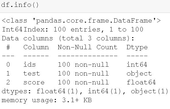
In the image above, we can see the structure of the dataframe. Our dataset contains 100 observations and three variables (columns). Furthermore, there are three different datatypes in the dataframe. First, we have an integer column (i.e., “ids”). This column contains the identifier for each individual in the study. Second, we have the column “test” which is of object data type and contains the information about the test time point. Finally, we have the “score” column where the dependent variable is. We can check the pairs by grouping the Pandas dataframe and calculating descriptive statistics:
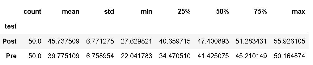
In the code chunk above, we grouped the data by “test” and selected the dependent variable, and got some descriptive statistics using the describe() method. If we want, we can use Pandas to count unique values in a column:
df['test'].value_counts()Code language: Python (python)This way, we got the information that we have as many observations in the post-test as in the pre-test. A quick note: before we continue to the next subsection, in which we subset the data, it has to be mentioned that you should check whether the dependent variable is normally distributed or not. This can be done by creating a histogram (e.g., with Pandas) and/or carrying out the Shapiro-Wilks test.
Subset the Data
Both methods, whether using SciPy or Pingouin, require that we have our dependent variable in two Python variables. Therefore, we will subset the data and select only the dependent variable. With our help, we have the query() method, and we will select a column using the brackets ([]):
b = df.query('test == "Pre"')['score']
a = df.query('test == "Post"')['score']Code language: Python (python)
Now, we have the variables a and b containing the dependent variable pairs we can use SciPy to do a paired sample t-test.
Python Paired Sample T-test using SciPy
Here’s how to carry out a paired sample t-test in Python using SciPy:
from scipy.stats import ttest_rel

# Python paired sample t-test
ttest_rel(a, b)Code language: Python (python)
In the code chunk above, we first started by importing ttest_rel(), the method we then used to carry out the dependent sample t-test. Furthermore, the two parameters we used were the data, containing the dependent variable, in the pairs (a, and b). Now, we can see by the results (image below) that the difference between the pre- and post-test is statistically significant.

In the next section, we will use Pingouin to carry out the paired t-test in Python.
How to Perform Paired Sample T-test in Python with Pingouin
Here is how to carry out the dependent samples t-test using the Python package Pingouin:
import pingouin as pt

# Python paired sample t-test:
pt.ttest(a, b, paired=True)Code language: Python (python)
There is not much to explain, about the code chunk above, but we started by importing pingouin. Next, we used the ttest() method and using our data. Notice how we used the paired parameter and set it to True. We did this because it is a paired sample t-test we wanted to carry out. Here is the output:
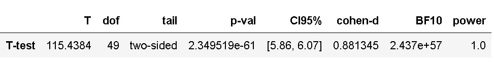
As you can see, we get more information when using Pingouin to do the paired t-test. Here we get all we need to continue and interpret the results. In the next section, before learning how to interpret the results, you can also watch a YouTube video explaining all the above (with some exceptions, of course):
Python Paired Sample T-test YouTube Video:
Here is the majority of the current blog post explained in a YouTube video:
How to Interpret the Results from a paired T-test
In this section, you will be given a short explanation of how to interpret the results from a paired t-test carried out with Python. Note we will focus on the results from Pingouin as they give us more information (e.g., degrees of freedom, effect size).
Interpreting the P-value
Now, the p-value of the test is smaller than 0.001, which is less than the significance level alpha (e.g., 0.05). This means that we can draw the conclusion that the quality of life increased when the participants conducted the post-test. Note, this can, of course, be due to other things than the intervention, but that’s another story.
Note that the p-value is the probability of getting an effect at least as extreme as the one in our data, assuming that the null hypothesis is true. Pp-values address only one question: how likely your collected data is, assuming a true null hypothesis? Notice, the p-value can never be used as support for the alternative hypothesis.
Interpreting Cohen’s D
Normally, we interpret Cohen’s D in terms of the relative strength of e.g. the treatment. Cohen (1988) suggested that d=0.2 is a ‘small’ effect size, 0.5 is a ‘medium’ effect size, and that 0.8 is a ‘large’ effect size. You can interpret this such as that iif two groups’ means don’t differ by 0.2 standard deviations or more, the difference is trivial, even if it is statistically significant.
Interpreting the Bayes Factor from Pingouin
When using Pingouin to carry out the paired t-test we also get the Bayes Factor. See this post for more information on how to interpret BF10.
How to Report the Results
This section will teach you how to report the results according to the APA guidelines. In our case, we can report the results from the t-test like this:
The results from the pre-test (M = 39.77, SD = 6.758) and post-test (M = 45.737, SD = 6.77) quality of life test suggest that the treatment resulted in an improvement in quality of life, t(49) = 115.4384, p < .01. Note, that the “quality of life test” is something made up, for this post (or there might be such a test, of course, that I don’t know of!).
In the final section, before the conclusion, you will learn how to visualize the data in two different ways: creating boxplots and violin plots.
How to Visualize the Data using Boxplots:
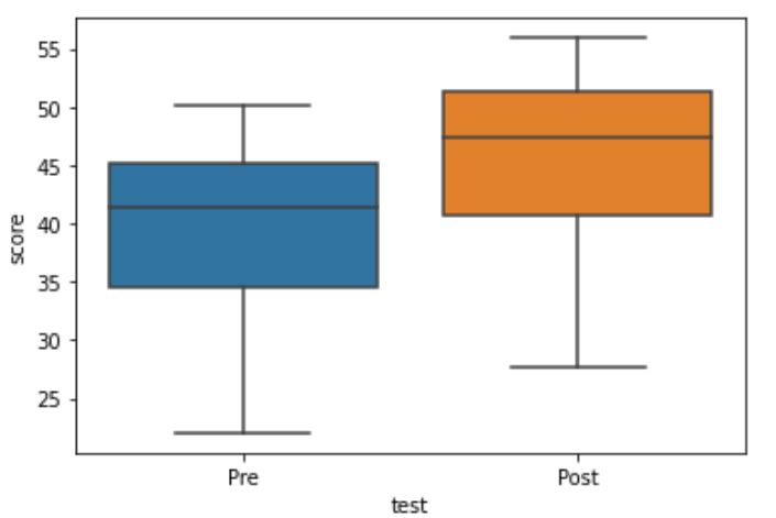
Here is how we can guide the interpretation of the paired t-test using boxplots:
import seaborn as sns

sns.boxplot(x='test', y='score', data=df)Code language: Python (python)
In the code chunk above, we imported seaborn (as sns), and used the boxplot method. First, we put the column that we want to display separate plots on the x-axis. Here is the resulting plot:
How to Visualize the Data using Violin Plots:
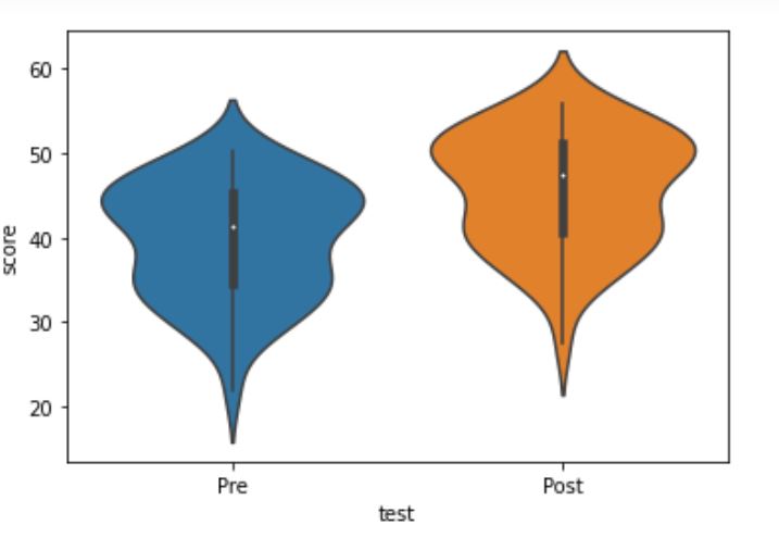
Here is another way to report the results from the t-test by creating a violin plot:
import seaborn as sns

sns.violinplot(x='test', y='score', data=df)Code language: Python (python)
Much like creating the box plot, we import seaborn and add the columns/variables we want as x- and y-axis’. Here is the resulting plot:
Alternative Data Analysis Methods in Python
As you may already be aware of, there are other ways to analyze data. For example, you can use Analysis of Variance (ANOVA) if there are more than two levels in the factorial (e.g. tests during the treatment, as well as pre- and post -tests) in the data. See the following posts about how to carry out ANOVA:
- Repeated Measures ANOVA in R and Python using afex & pingouin
- Two-way ANOVA for repeated measures using Python
- Repeated Measures ANOVA in Python using Statsmodels
Recently, machine learning methods have grown popular. See the following posts for more information:
Summary
In this post, you have learned two methods to perform a paired sample t-test. Specifically, in this post you have installed, and used, three Python packages for data analysis (Pandas, SciPy, and Pingouin). Furthermore, you have learned how to interpret and report the results from this statistical test, including data visualization using Seaborn. In the Resources and References section, you will find useful resources and references to learn more. As a final word: the Python package Pingouin will give you the most comprehensive result and that’s the package I’d choose to carry out many statistical methods in Python.
If you liked the post, please share it on your social media accounts and/or leave a comment below. Commenting is also a great way to give me suggestions. However, if you are looking for any help, please use other means of contact (see, e.g., the About or Contact pages).
Finally, support me and my content (much appreciated, especially if you use an AdBlocker): become a patron. Becoming a patron will give you access to a Discord channel in which you can ask questions and may get interactive feedback.
Additional Resources and References
Here are some useful peer-reviewed articles, blog posts, and books. Refer to these if you want to learn more about the t-test, p-value, effect size, and Bayes Factors.
Cohen, J. (1988). Statistical Power Analysis for the Behavioral Sciences (2nd ed.). Hillsdale, NJ: Lawrence Erlbaum Associates, Publishers.
It’s the Effect Size, Stupid – What effect size is and why it is important
Using Effect Size—or Why the P Value Is Not Enough.
Beyond Cohen’s d: Alternative Effect Size Measures for Between-Subject Designs (Paywalled).
A tutorial on testing hypotheses using the Bayes factor.