This post will teach you how to carry out the Kruskal-Wallis test in R. The Kruskal-Wallis test is a non-parametric statistical test used to determine whether there is a significant difference in the median values of two or more independent groups. This method is used when the analyzed data is not normally distributed, or the sample size is small. In addition, when the normality assumption is violated, the Kruskal-Wallis test is used instead of the traditional one-way analysis of variance (ANOVA).

Table of Contents
- Outline
- Requirements
- Kruskal-Wallis Test
- Simulating Example Datasets for Kruskal-Wallis Test in R
- Visualizing the Distribution of the Data using ggplot2
- Testing the Data for Normality using a Parametric Test
- The Kruskal-Wallis Test in R
- Interpreting the Kruskal-Wallis Test
- Visualizing the Results from the Kruskal-Wallis Test in R
- Post-Hoc Test: the Dunn Test
- Conclusion: Kruskal-Wallis test in R
- Additional Resources
Outline
This post is structured as follows. First, we start by answering some questions related to the Kruskal-Wallis test. Second, we learn about the requirements of this test and what you need to follow in this tutorial. Third, we will cover the test briefly. This section is followed by a data simulation section, which can be skipped if you are working with your data. In the fourth section, we will plot the distribution. Then we will carry out the Shapiro-Wilks test for normality and learn how to run the Kruska-Wallis test using R statistical environment. Finally, we will also look at a posthoc (Dunn) test on the same simulated data.
When the data being analyzed is not normally distributed, the Kruskal-Wallis test is used instead of traditional one-way ANOVA. In addition, it is also used when the sample size is small and the normality assumption cannot be met. In these circumstances, the Kruskal-Wallis test is preferable to an ANOVA because it is non-parametric and does not rely on the normality assumption.
The Kruskal-Wallis test compares the median values of two or more independent groups to see if they have a statistically significant difference. The rank of the observations is used to calculate the test statistic rather than the actual values. As a result, the Kruskal-Wallis test is classified as a non-parametric test.
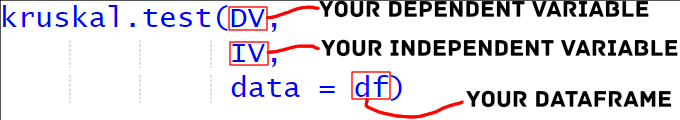
The Kruskal-Wallis test is very straightforward in R. We can use the kruskal.test() function. For example, we can use it using a formula: kruskal.test(DV ~ IV, dataframe).
Requirements
To run the Kruskal-Wallis test in R, the following requirements must be met:
- Data Format: The data must be in a format R can read, e.g., stored in a CSV or text file. Moreover, the data must also be organized into a dataframe, with each row representing an observation and each column representing a variable.
- Variable Names: The dataframe must include a variable representing each observation’s group membership (i.e., the independent variable) and a variable representing the measurement data (i.e., the dependent variable). Moreover, the variable names should be descriptive and meaningful, making understanding the data and results easier.
- Missing Data: Missing data must be handled appropriately. If missing data is present, it is recommended to either impute the missing values or remove the observations with missing data.
- Assumptions: The Kruskal-Wallis test does not assume the data is normally distributed. However, it does assume that the groups are independent and have equal variances. It is essential to check these assumptions before carrying out the test.
- R Environment: R statistical environment must be installed on the computer, and the required libraries must be loaded. This post will use the stats library to carry out the test. The ggplot2 library is also used to visualize data and check for normality. Finally, we also use the dunn.test package to carry out the Dunn post-hoc test.
Kruskal-Wallis Test
Null and Alternative Hypotheses
In the Kruskal-Wallis test, the null hypothesis states no significant difference between the analyzed groups’ median values. Moreover, according to the alternative hypothesis, there is a significant difference between the groups’ median values.
The Kruskal-Wallis test can be run in R using the stats package’s kruskal.test() function. The data must be passed as a vector or matrix to the function. Moreover, the grouping variable must be passed as a factor. The function returns the test statistic (H), p-value, degrees of freedom, and the test method. The output can be used to determine whether the null hypothesis can be rejected. If the null hypothesis is rejected, there is a significant difference between the median values of the groups under consideration.
The coin package is another option for performing the Kruskal-Wallis test in R. This package’s kruskal_test() function can be used to perform the test. This function, which also accepts data and grouping variables as arguments, returns the test statistic, p-value, and degrees of freedom. As previously mentioned, in this post, we will use the function from the stats package.
The test statistic (i.e., H) is computed using the rank of the observations and compared to a critical value from a degree of freedom chi-squared distribution. If the calculated value of the test statistic is greater than the critical value, the null hypothesis is rejected. We can then conclude that there is a significant difference between the groups’ median values.
Simulating Example Datasets for Kruskal-Wallis Test in R
To demonstrate the use of the Kruskal-Wallis test in R, we will simulate both skewed and unbalanced data from the field of Cognitive Psychology in this R tutorial. First, we will use ggplot2 to visualize the data because it does not meet the normality assumption. We will also use the Shapiro-Wilks (a parametric test) to help interpret the data’s non-normality.
Step 1: Load Required Libraries
The first step is to load the needed library, which is the ggplot2 package:
library(ggplot2)Code language: R (r)Step 2: Generate Sample Data
We will generate sample data using the stats package’s rnorm() function. Moreover, we will generate three data groups with different means and standard deviations to simulate skewed data.
set.seed(323)
group1 <- rnorm(100, mean = 107, sd = 29)^2
group2 <- rnorm(79, mean = 89, sd = 17)^2
group3 <- rnorm(66, mean = 68, sd = 35)^2Code language: R (r)
Note that we are setting the seed to enable simulation replication later. Moreover, we use the ^ to get positively skewed data.
Step 3: Combine Groups into a Single Dataset and Add a Grouping Variable
Next, using the c() function, we will combine the three data groups into a single dataset.
data <- c(group1, group2, group3)Code language: R (r)Note you can also find the z-score in R to standardize data. Doing this may transform the data to a normal distribution.
The following step will create a grouping variable that will indicate which observations belong to which group. For example, the observations in groups 1, 2, and 3 will be assigned the values 1, 2, and 3, respectively.
grouping <- rep(c(1,2,3), c(100, 79, 66))Code language: R (r)In the code chunk above, we used the rep() function to generate a sequence in R.
Step 4: Combine Data and Grouping Variable into a Dataframe
Next, we will use the data.frame() function combines the data and grouping variables into a single data frame.
df <- data.frame(data, grouping)Code language: R (r)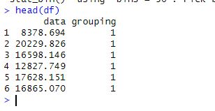
Other options can be read in the following posts:
- Learn How to Convert Matrix to dataframe in R with base functions & tibble
- How to Read and Write Stata (.dta) Files in R with Haven
- R Excel Tutorial: How to Read and Write xlsx files in R
Visualizing the Distribution of the Data using ggplot2
In this part of the tutorial, we will visualize the simulated data to inspect the distribution visually. In the first step, we will visualize data. After visualizing the data (i.e., creating a histogram), we will interpret the histogram.
Step 1: Plot the Data using ggplot2
We will use the ggplot() function from the ggplot2 package to plot the data and visualize its distribution. In addition, the geom_histogram() function will be used to create a histogram of the data, and the facet_wrap() function will be used to separate the histograms by group.
ggplot(df, aes(x = data, fill = factor(grouping))) +
    geom_histogram(alpha = 0.5, position = "dodge") +
    facet_wrap(~grouping, ncol = 3) +
    labs(x = "Data", y = "Frequency") +
    scale_fill_brewer(palette = "Paired") +
    theme_bw()Code language: R (r)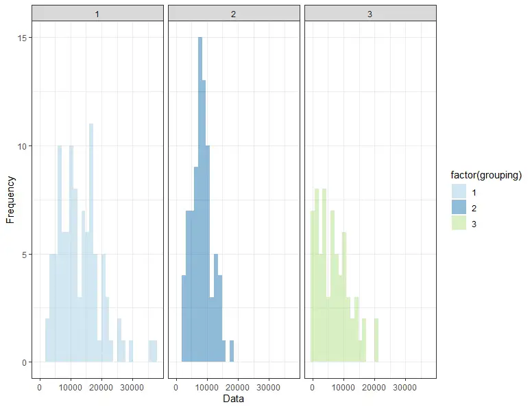
For more data visualization tutorials:
Step 2: Interpret the Plot
The histogram demonstrates that the data is not normally distributed and is skewed, with the means and standard deviations of the different groups differing. However, it may be hard to interpret histograms. Therefore, in the next section, we will examine the Shapiro-Wilks test.
Testing the Data for Normality using a Parametric Test
We will use the stats package’s function to perform the Shapiro-Wilk normality test on the data. The Shapiro-Wilk test is a popular parametric test for determining whether a sample is normally distributed.
shapiro.test(df$data)Code language: R (r)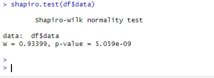
The p-value for the test is less than 0.05, indicating that the data is not normally distributed. This backs up our visual interpretation of the data from the ggplot2 plot, which revealed that it is skewed and unbalanced. Other tests for normality can be conducted in R:
Finally, we successfully simulated and visualized skewed and unbalanced datasets from cognitive psychology. The Shapiro-Wilk test and the ggplot2 plot showed that the data did not meet the normality assumption. Because it does not require the normality assumption, the Kruskal-Wallis test can be used to analyze this data type, making it a useful tool for comparing the median values of multiple groups in situations where the data is skewed and unbalanced.
The Kruskal-Wallis Test in R
Carrying out the Kruskal-Wallis test in R is a straightforward process involving only one step (i.e. if we already have our data loaded). To carry out the test in R, we use the kruskal.test function. The function requires a single argument, the name of the variable we want to test. In this case, our variable is named data.
kruskal.test(data ~ grouping, data=df)
Code language: R (r)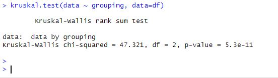
Interpreting the Kruskal-Wallis Test
The test results tell us a lot about the significance of the differences between the median values of each group. Among the outcomes are:
- The test statistic assesses the strength of the groups’ relationship.
- The degrees of freedom are a measure of data variability.
- The p-value represents the likelihood of obtaining a test statistic as extreme as the one observed if the null hypothesis is true.
Remember, according to the null hypothesis, there is no significant difference between the median values of each group. If the p-value is less than 0.05, we reject the null hypothesis and conclude that the median values of the groups differ significantly.
In our case, the p-value is 0.0001, which is less than 0.05, indicating that the median values of the groups differ significantly.
Visualizing the Results from the Kruskal-Wallis Test in R
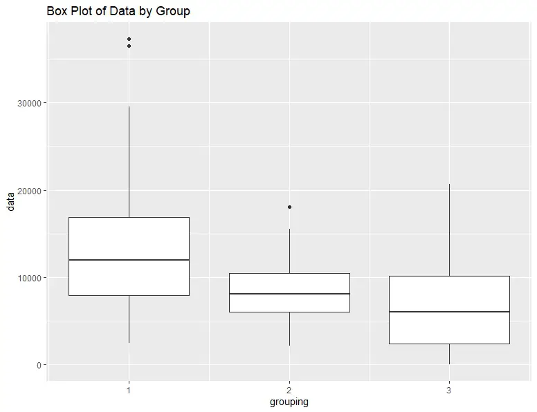
Finally, we can visualize the results by creating a box plot of the data. A box plot is a convenient way to visualize the data distribution, including the median, quartiles, and outliers. Again, we will use ggplot2:
ggplot(df, aes(x=grouping, y=data, group=grouping)) +
    geom_boxplot() +
    ggtitle("Box Plot of Data by Group")Code language: R (r)
The resulting box plot shows that the median values of each group are significantly different, as indicated by the results from the test.
Another option to visualize the data is by creating a violin plot. See the post How to Create a Violin Plot in R with ggplot2 and Customize it for more information.
Post-Hoc Test: the Dunn Test
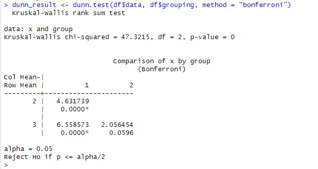
The Dunn test is a post hoc test used to determine which group pairs significantly differ from each other after the Kruskal-Wallis test. The Dunn test is a non-parametric test that makes no assumptions about the data’s underlying distribution.
The difference between the mean ranks of two groups divided by the standard deviation of the rank scores is the Dunn test statistic. This test statistic is then compared to a critical value obtained from a table or a software package to determine whether the groups differ significantly.
# Load the required libraries (install it if you need to)
library(dunn.test)

# Conduct the Dunn test post-hoc test
dunn_result <- dunn.test(df$data, df$grouping, method = "bonferroni")

# Print the results
print(dunn_result)Code language: R (r)
In the code chunk above, we first load the required library, dunn.test. We then conduct the Dunn test using the dunn.test function. The results of the Dunn test are printed on the console. The method argument specifies the correction method to use, in this case, the “bonferroni” correction. The dunn_result object contains several components, including the test statistic, p-value, and which pairs of groups are significantly different.
Conclusion: Kruskal-Wallis test in R
In conclusion, the Kruskal-Wallis test is useful for comparing the median values of multiple groups in situations where the data is skewed and unbalanced. The test is straightforward to carry out in R, and the results provide important information about the significance of the differences between the groups. Visualizing the results through a box plot is a convenient way to better understand the data and test results.
Please comment if you know of any other R packages or functions that can perform the Kruskal-Wallis test in R. You are welcome to suggest topics for future blog posts, correct any errors in my blog posts, or let me know if you found the post helpful. That is, I invite you to leave a comment below!
Additional Resources
Here are some other blog posts found on this blog that you might find helpful.
- How to use $ in R: 6 Examples – list & dataframe (dollar sign operator)
- Learn How to use %in% in R: 7 Example Uses of the Operator
- How to Add a Column to a Dataframe in R with tibble & dplyr
- R: Add a Column to Dataframe Based on Other Columns with dplyr
- How to Remove a Column in R using dplyr (by name and index)
- R Count the Number of Occurrences in a Column using dplyr
- How to Add an Empty Column to a Dataframe in R (with tibble)