In this tutorial, you will learn how to calculate descriptive statistics in R, a fundamental tool for data analysis. Descriptive statistics provide an overview of the key characteristics of a dataset, including measures of central tendency, variability, and distribution. These statistics help us to understand the distribution of data and can be used to identify patterns and relationships within the data.
Table of Contents
- Outline
- Why Descriptive Statistics?
- Installing the R-packages
- Descriptive statistics in R
- Summary statistics in R: Measures of Central Tendency
- Descriptive Statistics: Measures of Variability in R
- Summary Statistics in R using psych
- Descriptive Statistics in R with dplyr
- LaTeX Table with Descriptive Statistics
- Saving Descriptive Statistics in R to a CSV File
- Conclusion: Descriptive Statistics in R
- Tutorials
Outline
We will start by installing the necessary R-packages and importing data. Then, we will explore how to calculate measures of central tendency, such as the mean and median, and how to calculate them by one or two groups. We will also cover less commonly used measures of central tendency, such as geometric, harmonic, and trimmed mean.
Next, we will dive into measures of variability, including the standard deviation, interquartile range, and quantiles. These measures help us understand the data’s spread and can be used to identify outliers or unusual observations.
We will also explore how to use the psych and dplyr packages to calculate summary and descriptive statistics by group. Additionally, we will learn how to create a LaTeX table with descriptive statistics and how to save descriptive statistics to a CSV file for future analysis.
By the end of this tutorial, you will have a solid understanding of using R to calculate and interpret descriptive statistics. Whether new to R or looking to expand your data analysis skills, this tutorial will provide the knowledge and tools needed to work confidently with descriptive statistics in R.
Note, in a recent post, you learn how to quickly explore your data with one of Tukey’s exploratory data analysis methods:
Why Descriptive Statistics?
Calculating descriptive statistics in R is crucial in any data analysis process. Descriptive statistics provide a concise summary of a dataset’s key characteristics, helping us understand its distribution and identify patterns and relationships within the data.
There are, of course, plenty of useful r-packages for data manipulation and summary statistics. In this post, we will mainly work with the base R functions and the psych and Tidyverse packages. Tidyverse comes with a bunch of handy packages that you can use to, for example, add an empty column to the dataframe.
Installing the R-packages
As mentioned in the previous section, we are, in this descriptive statistics with R post, going to work with some r-packages. If they’re not installed, the following commands will install them.
list.of.packages <- c("tidyverse", "psych", "knitr", "kableExtra")
new.packages <- list.of.packages[!(list.of.packages %in% installed.packages()[,"Package"])]
if(length(new.packages)) install.packages(new.packages)Code language: R (r)
In the code chunk above, we created the vector with the packages we wanted to install. Second, we created a new vector that matches value (with the %in% operator in R). Finally, we only installed the packages that were not installed already!
In this summary statistics in R tutorial, we will start by calculating descriptive statistics and some variance measures. After that, we continue with the most common ways to report the central tendency (i.e., the mean, the median). Finally, we will calculate the harmonic, geometric, and trimmed mean.
Descriptive statistics in R
In this section, we will start by calculating some demographic statistics for our data. Furthermore, we will calculate the missing values by group, the % of missing values by group, the mean age, age range, and such.
Import Data
First, however, we are going to read an xlsx file using R (it can be downloaded here):
library(readxl)
play_df <- read_excel("../SimData/play_data.xlsx")Code language: R (r)
Note, data can be stored in a range of different formats. For instance, we can also read a .dta (Stata) file, and a SPSS (.sav) with R.
Before calculating some summary statistics, we can look at the first five rows of our data by typing head(play_df). Here is what the data looks like:
Second, as we can see in the Gender column, it is coded as 0 (and 1), and we are going to recode the values to “Male” and “Female”. We are going to use the recode function. If we want or need to, we can also remove a column. Alternatively, we can also select the columns we want to use when calculating the summary statistics.
library(tidyverse)

# Renaming variables:
play_df$Gender <- play_df$Gender %>%
  recode("0" = "Male",
         "1" = "Female")Code language: R (r)
Descriptive Statistics: e.g., mean age, range, and standard deviation
In this section, we are going to summarize the information about the participants of the study. That is, we will calculate the mean and standard deviation in terms of age and the age range. Here, we use the Tidyverse package, again, and the summarise function:
require(tidyverse)

# Summarizing the dataframe:
play_df %>%
  summarise(sd = sd(Age, na.rm = T),
            mean = mean(Age, na.rm = T),
            range = paste(min(Age, na.rm = T), "-", max(Age, na.rm = T)),
            n = sum(!is.na(Age)))Code language: R (r)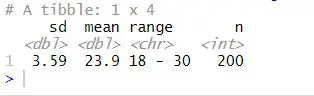
In the code chunk above, we calculated some summary statistics about the sample. Note we used the na.rm = T because there might be missing values in the variable Age. To create the age range variable, we take the min and the max of the variable Age. Notice that we used the paste function to create the range.
Descriptive Statistics in R by Group: mean age, age range, standard deviation
Now, we will group the data and calculate the mean, standard deviation, age range, and how many are in each group. In the code chunk below, all we have done is add the group_by method and added “Gender” to that.
library(tidyverse)

# Summarizing by group:
play_df %>% group_by(Gender) %>%
  summarise(sd = sd(Age, na.rm = T),
            mean = mean(Age, na.rm = T),
            range = paste(min(Age, na.rm = T), "-", max(Age, na.rm = T)),
            n = sum(!is.na(Age)))Code language: R (r)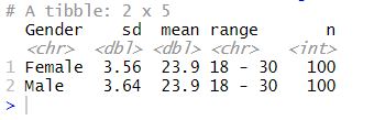
Summary statistics in R: Measures of Central Tendency
In this part of the R descriptive statistics tutorial, we will focus on the measures of central tendency. The central tendency is something we calculate because we often want to know about the “average” or “middle” of our data. The two most commonly used measures of central tendency can easily be obtained using R; the mean and the median.
Calculate the Mean in R
In the previous section, we calculated summary statistics (e.g., mean, standard deviation, range) in one go. However, if we are only interested in one summary statistic, we can calculate them separately. First, if we only want to calculate the mean of one of our variables, we can use the mean function. Note, here we are interested in calculating the summary statistics for the dependent variable “RT”:
# Calculating mean value:
mean(play_df$RT, na.rm = T)
# Output: [1] 0.4963685Code language: R (r)
Calculate the Mean by One Group
Second, when we use Tidyverse group_by and summarise functions, we add the mean function. Note, this is very similar to what we did previously.
# Mean by Gender:
play_df %>% group_by(Gender) %>%
  summarise(RT = mean(RT, na.rm = T))Code language: R (r)
Calculate the mean by Two Groups
Third, if we want to calculate the mean by two groups we add a group to the group_by function:
# Calculating mean by multiple (i.e, 2) groups:
play_df %>% group_by(Gender, Day) %>%
  summarise(RT = mean(RT, na.rm = T))Code language: R (r)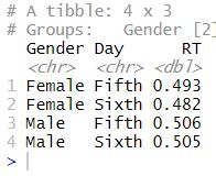
Geometric, Harmonic, & Trimmed Mean in R
In this section, we will use the R-package psych to calculate the geometric, harmonic, and trimmed mean in R. Many times; it may be better to calculate the geometric and harmonic mean when doing summary statistics. In R, these two descriptive statistics can be obtained using the summarise function together with the functions geometric.mean and harmonic.mean (from psych).
Geometric Mean in R
In this section, we will calculate the geometric mean in R. One very nice thing when working with summarise is that we can input any function, from another package, that we need to use. In the following code chunk, we are going to use the geometric.mean function from the psych package to calculate the geometric mean.
# Calculating geometric mean by multiple groups:
play_df %>% group_by(Gender, Day) %>%
  summarise("Geometric Mean" = psych::geometric.mean(RT, na.rm = T))Code language: R (r)
Harmonic Mean in R
In this R summary statistics example, we use summarise together with harmonic.mean to get the harmonic mean in R:
# Harmonic mean grouped by multiple groups
play_df %>% group_by(Gender, Day) %>%
  summarise("Harmonic Mean" = psych::harmonic.mean(RT, na.rm = T))</code></pre>Code language: R (r)
Trimmed Mean in R
In this section, we are going to calculate the trimmed mean. This can be done using the mean function. All we do is use the trim=.2:
play_df %>% group_by(Gender, Day) %>%
  summarise("Harmonic Mean" = mean(RT, trim=0.2, na.rm = T))Code language: R (r)
Get the Median in R
In this section, we will calculate the median using R. It’s as easy as calculating the mean and just use the function called median.
median(play_df$RT, na.rm = T)Code language: R (r)Median by Groups in R
Of course, we often want the median, as well, calculated by group (e.g. categorical variable) and if we want to calculate the median by group we use group_by, again, and summarise:
play_df %>% group_by(Gender, Day) %>%
  summarise(Mean = median(RT, na.rm = T))Code language: R (r)
Measures of Central Tendencies in One Tibble (Mean, Median, Harmonic, Geometric, and Trimmed)
Now, most of the time we want to get all the measures of central tendency (or all summary statistics we calculate in R) in the same output. We can, of course, get all the data in the same output using summarise. In the descriptive statistics in R example below, the standard deviation (sd), mean, median, harmonic mean, geometric mean, and trimmed mean are all in the same output.
play_df %>%  group_by(Gender, Day) %>%
  summarise(SD = sd(RT, na.rm = T),
            Mean = mean(RT, na.rm = T),
            Median = median(RT, na.rm = T),
            "Trimmed Mean" = mean(RT, trim = 0.2, na.rm = T),
            "Geometric Mean" = psych::geometric.mean(RT, na.rm = T),
            "Harmonic Mean" = psych::harmonic.mean(RT, na.rm = T))Code language: PHP (php)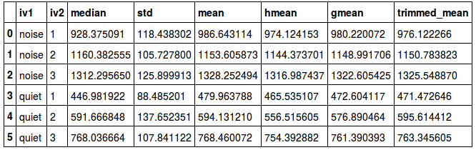
Descriptive Statistics: Measures of Variability in R
Central tendency (e.g., the mean & median) is not the only type of descriptive statistic that we want to calculate. Most of the time, we also want to have a look at a measure of the variability of our data.
Standard deviation in R
In this section, we are going to calculate the standard deviation using R. We have actually already done this using the function sd.
sd(play_df$RT, na.rm = T)Code language: R (r)If we want to calculate the standard deviation by groups this is, again, doable using the group_by and summarise functions.
play_df %>% group_by(Gender, Day) %>%
  summarise("SD" = sd(RT, na.rm = T))Code language: R (r)
Interquartile Range in R
In this descriptive statistics in R example, we will use IQR to calculate the interquartile range in R.
IQR(play_df$RT, na.rm = T)Code language: R (r)Quantiles in R
We can also calculate quantiles. Here, we only do this by groups and create a custom function (see this post for the original code adapted in the example below) to do this together with summarise_at.
p <- c(0.25, 0.5, 0.75)

p_funs <- map(p, ~partial(quantile, probs = .x, na.rm = TRUE)) %>%
  set_names(nm = p)

play_df %>%  group_by(Gender, Day) %>%
  summarise_at(vars(RT), lst(!!!p_funs))Code language: R (r)
Calculate Variance in R
We will calculate the variance in the last section of this descriptive statistics in R tutorial. Furthermore, In R, the variance is easy to calculate using R. In the summary statistics in the R example below, we will use the var function.
var(play_df$RT, na.rm = T)Code language: R (r)Now, we are going to calculate the descriptive statistic variance by groups.
play_df %>% group_by(Gender, Day) %>%
  summarise(Variance = var(RT, na.rm = T))Code language: R (r)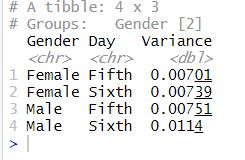
For a more detailed description of variation calculation in R:
After calculating the descriptive statistics, we can also visualize the data. Another step in the data analysis pipeline may be dummy coding. A more recent post covered how to create dummy variables in R.
Summary Statistics in R using psych
In this section, we will use the r-package psych to calculate most of the descriptive statistics we calculated above. Here, we will use the function describeBy to calculate the standard deviation, median, mean, interquartile range, trimmed mean range, skewness, kurtosis, standard error, and quantiles.
library(psych)
with(play_df, describeBy(RT, group = list(Gender, Day),
                         IQR = T, quant = c(0.25, 0.50, 0.75)))Code language: R (r)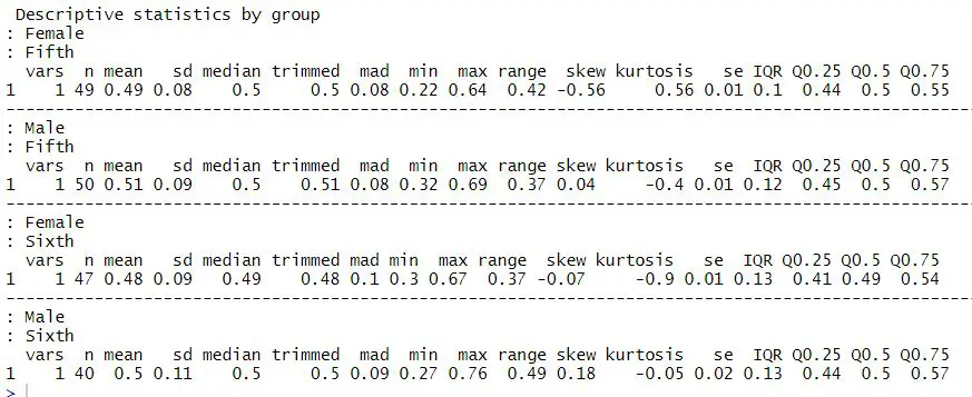
Descriptive Statistics in R with dplyr
In this section, we will calculate the summary statistics above, using dplyr and the group_by() and summarise() functions. Furthermore, we are saving this table and will create a latex table using the kable function from the knitr package.
tbl <- play_df %>%  group_by(Gender, Day) %>%
  summarise(SD = sd(RT, na.rm = T),
            Mean = mean(RT, na.rm = T),
            Median = median(RT, na.rm = T),
            "Trimmed Mean" = mean(RT, trim = 0.2, na.rm = T),
            "Geometric Mean" = psych::geometric.mean(RT, na.rm = T),
            "Harmonic Mean" = psych::harmonic.mean(RT, na.rm = T),
            IQR = IQR(RT, na.rm = T),
            "%25 Q" = quantile(RT, .25, na.rm = T),
            "%50 Q" = quantile(RT, .5, na.rm = T),
            "%75 Q" = quantile(RT, .75, na.rm = T))Code language: R (r)
LaTeX Table with Descriptive Statistics
Now, we are ready to use kable to create a latex table. In the code chunk below, we load kableExtra and knitr. Kable is used to creating the latex table, and kable_styling is to scale the table down, so it fits a PDF created with RMarkdown.
library(kableExtra)
library(knitr)

kable(tbl, format = "latex",
      digits=2, booktabs = TRUE) %>%
          kable_styling(latex_options = "scale_down")Code language: R (r)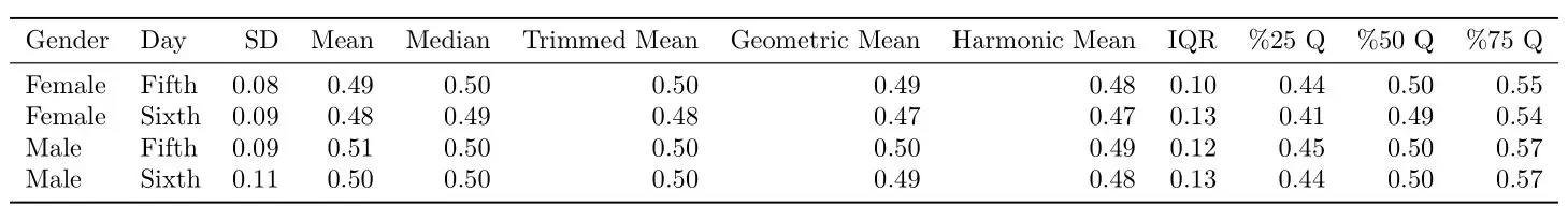
Saving Descriptive Statistics in R to a CSV File
If we want to save our descriptive statistics, calculated in R, we can use the Tidyverse write_excel_csv function. In the example below, we are saving the R tibble tbl created earlier to a .csv file:
write_excel_csv(tbl, "descriptive_stats.csv")Code language: R (r)
The next step in the data analysis pipeline would be to visualize the data to explore possible relationships further. See the scatter plot in R with ggplot2 tutorial for more information on data visualization in R.
Conclusion: Descriptive Statistics in R
In this post, we have learned how to describe our data. More specifically, we have learned how to calculate measures of central tendency (mean, median, etc.), variability (standard deviation), and more. Furthermore, we computed summary statistics using R and saved them as a latex table and a CSV file.
Tutorials
Here are plenty more posts to guide you on your learning journey:
- Modulo in R: Practical Example using the %% Operator
- How to Create a Word Cloud in R
- How to Rename Column (or Columns) in R with dplyr
- Correlation in R: Coefficients, Visualizations, & Matrix Analysis
- Coefficient of Variation in R