Correlation Matrix in R: A Hands-On Guide for Practical Analysis

In this post, we will look deeper into how to create a correlation matrix in R. Building on our previous exploration of how to conduct correlation analysis in R more generally; this guide goes into the specifics of correlation matrices, a powerful tool in data analysis. A correlation matrix provides a comprehensive view of relationships between variables, making it a crucial asset in understanding complex datasets. In this post, we will adopt a hands-on and practical approach, emphasizing the application of correlation matrices in R. Whether you are familiar with basic correlation analysis or just starting, this post will equip you with practical skills for effective data interpretation and visualization.

Outline
Prerequisites
Synthetic Data
Creating a Correlation Matrix in R
- Base R Functions for Correlation Matrix
- Creating a Correlation Matrix in R using the corrr package
Visualizing Correlation Matrix in R
- Base R Method
- Visualizing a Correlation Matrix using the corrr Package
Saving Correlation Matrix as APA 7 Table
Other packages
Base R vs. the corrr package
Conclusion
Resources

Outline

The structure of the post is as follows. First, we establish the prerequisites, ensuring readers have a foundational understanding of R and basic statistical concepts. Moving on, we learn the practical side of correlation analysis with synthetic data, providing a hands-on approach.

In the core sections, we explore two methods of creating a correlation matrix in R. Initially, we leverage base R functions, demonstrating their utility and explaining their parameters. Subsequently, we introduce the corrr package, highlighting its user-friendly functions that streamline the process.

Transitioning to visualization, we cover both base R methods and those facilitated by the corrr package. The post then get into the crucial aspect of saving a correlation matrix in compliance with APA 7 standards using the apaTables package.

Briefly, we touch upon other packages that offer additional functionalities for correlation analysis, expanding readers’ awareness of available tools. We then consider the pros and cons of using base R versus the corrr package for correlation tasks.

The post concludes by summarizing the key takeaways, emphasizing the practical aspects covered, and encouraging readers to adopt the approach that best suits their preferences and analytical needs.

Prerequisites

Before reading this hands-on R tutorial on creating correlation matrices, it is crucial to have a basic understanding of correlation analysis. Please familiarize yourself with what correlation is, when to use it, and the nature of data suitable for correlation analysis. Ensure that your data aligns with correlation assumptions.

For those planning to use the corrr package and tidyverse functions, make sure to install them using the following code:

# Install corrr and tidyverse packages
install.packages("corrr")
install.packages("tidyverse")  # or "dplyr"
Code language: PHP (php)

Additionally, consider checking your R version using the sessionInfo() function and update R if needed. While not mandatory, a familiarity with tidyverse packages such as dplyr can be advantageous. These tools facilitate tasks like renaming factor levels, renaming variables, creating dummy variables, counting unique occurrences, and summarizing data by rows and columns.

Synthetic Data

Here is a synthetic dataset that we will use to create and visualize a correlation matrix in R:

# Set seed for reproducibility
set.seed(323)

# Generate a dataset with 5 correlated variables
n <- 100  

# Variables 1 to 3: Correlated 
var1 <- rnorm(n)
var2 <- 0.25 * var1 + rnorm(n, sd = 0.2)
var3 <- 0.25 * var1 + rnorm(n, sd = 0.2)

# Variables 4 and 5: Correlated with each other but independent of Variables 1 to 3
var4 <- rnorm(n)
var5 <- 0.3 * var4 + rnorm(n, sd = 0.2)

# Combine into a data frame
psych_data <- data.frame(Var1 = var1, Var2 = var2, Var3 = var3, Var4 = var4, Var5 = var5)Code language: R (r)

In the code chunk above, we create a reproducible dataset with five correlated variables representing everyday hearing difficulties. Variables Var1, Var2, and Var3 are interrelated, simulating measurements of a single hearing-related problem. Meanwhile, variables Var4 and Var5 correlate, indicating measurements related to a distinct hearing difficulty. The magnitudes of the correlation coefficients have been adjusted to reflect real-life scenarios, contributing to a synthetic dataset suitable for exploring correlation matrices.

Creating a Correlation Matrix in R

In this section, we will explore two distinct methods to generate a correlation matrix in R, starting with base R functions and using the corrr package for enhanced usability.

Base R Functions for Correlation Matrix

We will use fundamental base R functions to initiate our exploration, primarily focusing on the cor() function. This versatile function calculates the correlation matrix for a given dataset. We will look at its parameters, discussing how adjustments can be made to tailor the analysis to specific needs.

R’s cor() function parameters include:

x: A numeric matrix or data frame containing the variables for which correlations are to be computed.
y: An optional second numeric matrix or data frame. If provided, the function calculates correlations between corresponding columns in both matrices.
use: A character indicating the handling of missing values. Options include “everything,” “all.obs,” “complete.obs,” and “pairwise.complete.obs.”
method: A character vector specifying the correlation coefficient to be computed. Options include “pearson” for Pearson’s correlation (default), “kendall” for Kendall’s tau, and “Spearman” for Spearman’s rank correlation.

When working with a single matrix (x), the y parameter is not required, making the function particularly efficient for matrix-to-matrix correlation calculations, which is the focus of the current post.

Next, we will use the synthetic psych_data dataset representing everyday hearing difficulties to demonstrate the creation of a correlation matrix.

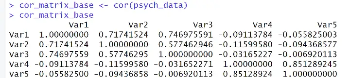
# Calculate the correlation matrix using base R
cor_matrix_base <- cor(psych_data)Code language: R (r)

To enhance readability, we can focus on either the upper or lower triangle of the correlation matrix.

Here is how to get the upper triangle:


# Get upper triangle
upper_triangle <- cor_matrix[upper.tri(cor_matrix)]Code language: CSS (css)

In the code chunk above, we manipulate the correlation matrix cor_matrix_base to obtain only its upper triangle. The lower.tri() function, when applied to the cor_matrix_base matrix, returns a logical matrix where the lower triangle is marked as TRUE and the upper triangle as FALSE. By setting the elements in the lower triangle to NA in the original correlation matrix using square bracket indexing, we effectively retain only the upper triangle of the correlation matrix.

Alternatively, we can extract the lower triangle using a similar approach. Here is how to get the lower triangle:

# Get upper triangle
lower_triangle <- cor_matrix[lower.tri(cor_matrix)]Code language: CSS (css)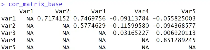

In the code chunk above, notice how we used the upper.tri() function instead of the lower.tri(). This will get us the lower triangle of the matrix. The following section will use the corrr package to get the correlation matrix.

Creating a Correlation Matrix in R using the corrr package

The corrr package offers a streamlined approach to correlation matrix computation in R. This package’s correlate() function is designed for enhanced simplicity and flexibility. Key parameters include:

x: A numeric matrix or data frame containing the variables for correlation computation.
y: An optional second numeric matrix or data frame. If specified, correlations are computed between corresponding columns in both matrices.
use: A character indicating the handling of missing values, similar to the base R cor() function.
method: A character vector specifying the desired correlation coefficient method (default is “Pearson”).
diagonal: An option to set diagonal values explicitly.
quiet: A logical indication of whether to suppress messages during computation.

# Load the corrr library:
library(corrr)

# Load synthetic data
psych_data <- read.csv("path_to_your_file.csv")

# Calculate and display the upper triangle using corrr
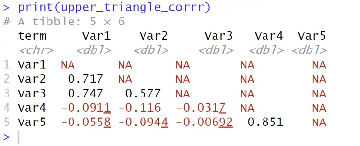
corrr_result <- correlate(psych_data)
upper_triangle_corrr <- corrr_result %>%
  shave()Code language: R (r)

In the code chunk above, we showcase the streamlined creation of a correlation matrix using the correlate() function from the corrr package. After creating the matrix, the pipe operator (%>% from dplyr) facilitates efficient data manipulation. Finally, to extract the upper triangle for easier interpretation, we used the shave() function. The code demonstrates the simplicity and utility of the corrr package for correlation analysis in R.

correlation matrix created with the R-package corrr

We can set the upper parameter to FALSE, allowing us to obtain the lower triangle instead.

Visualizing Correlation Matrix in R

This section will briefly look at examples of using base R and the corrr package to visualize our correlation matrices in R.

Base R Method

Visualizing correlation matrices is a good tool for gaining insights into variable relationships. In base R, we can, for example, use the pairs() function to create scatterplot matrices, providing a comprehensive view of pairwise correlations. Let us showcase this approach using our synthetic dataset on everyday hearing difficulties.

# Create scatterplot matrix using pairs()
pairs(psych_data)Code language: PHP (php)

In the code chunk above, we create a scatterplot matrix using the pairs() function in base R to explore the relationships among variables in the psych_data dataset visually.

This visualization technique provides an interactive and comprehensive representation of pairwise correlations, facilitating the identification of patterns and trends within the hearing-related variables.

Visualizing a Correlation Matrix using the corrr Package

The corrr package provides a convenient set of visualization tools for correlation matrices. Leveraging the network_plot() function allows us to create an informative network plot, emphasizing the strength and direction of correlations.

network_plot(corrr_result)Code language: R (r)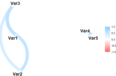

When visualizing correlation matrices in R, an alternative approach to the network plot provided by the corrr package using the rplot() function. This function offers a distinct visual representation, allowing us to explore relationships differently. Let us consider an example using our psych_data dataset on everyday hearing difficulties:

psych_data %>% correlate() %>%
  shave() %>%
  rplot()

In the code chunk above, we use the corrr package to generate a correlation matrix from the psych_data dataset. The correlate() function computes the correlation matrix, and shave() extracts the lower triangle. Finally, rplot() is employed to create a correlation plot, visually representing the relationships between variables in the dataset.

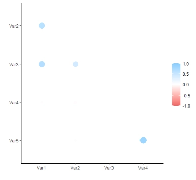
This streamlined sequence of functions offers a concise and efficient approach to compute and visualize the correlation matrix in R.

Saving Correlation Matrix as APA 7 Table

Presenting correlation results in academic writing requires adherence to specific standards, such as those outlined in APA 7. We can achieve this in R by exporting correlation matrices using the apaTables package, ensuring the generated tables meet APA 7 guidelines.

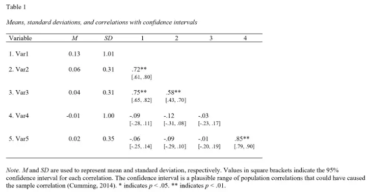
Let us first consider the apaTables package and its apa.cor.table() function. This function facilitates the creation of APA-style correlation tables with customizable options. For instance, here is how to create an APA correlation table:

apa.cor.table(psych_data, filename = "APA_Correlation_Table.doc", table.number = 1)
Code language: R (r)

In the code chunk above, we use the apa.cor.table() function to export our correlation matrix to a document titled “APA_Correlation_Table.doc.” Using apaTables provides a seamless process for creating publication-ready correlation tables.

Other packages

In addition to the corrr package, other valuable R packages enhance the capabilities of correlation analysis. The correlation package stands out for its ability to provide p-values alongside correlation coefficients, offering a comprehensive statistical assessment of relationships in the data. As part of the easystats package, correlation analysis is seamlessly integrated with various handy functions. These functions include the ease of creating insightful scatter plots in R, aiding in visualizing bivariate relationships.

Furthermore, the corrr package is complemented by other packages like Hmisc, which provides functions for correlation analysis and multiple imputation. The ggcorrplot package, based on ggplot2, is notable for creating visually appealing correlation plots. Similarly, the psych package is a robust tool for comprehensive correlation analysis, offering various functions for both exploratory and confirmatory approaches. With these diverse packages, R users have many options to conduct, visualize, and interpret correlation analyses efficiently.

Base R vs. the corrr package

Choosing between base R and the corrr package for creating a correlation matrix involves weighing the pros and cons. Base R, a fundamental part of the R language, ensures independence from external package maintenance. Using cor() thus makes it a robust and reliable option, particularly for users concerned about package longevity.

However, the corrr package introduces user-friendly functions that streamline the process, making it more accessible for those less experienced with coding. Its functions, such as focus() and stretch(), enhance interpretability, and extend functionality beyond what base R offers. Additionally, the corrr package’s compatibility with the tidyverse ecosystem and active development contribute to its appeal.

In contrast, base R requires users to navigate through additional steps and may have a steeper learning curve for beginners. While it provides core functionality, users might find the corrr package more intuitive and efficient for tasks related to correlation analysis. Ultimately, the choice depends on the user’s preference, familiarity with R, and specific requirements for their analytical workflow.

Conclusion

In conclusion, this guide has equipped you with the tools and insights to perform correlation analysis in R. From understanding prerequisites to creating, visualizing, and saving correlation matrices, we have navigated the intricacies of this statistical process. Whether opting for base R or leveraging the user-friendly corrr package, you now possess the knowledge to choose the method that best aligns with your workflow.

Remember to consider the APA 7 guidelines for presenting correlation results and the wealth of options provided by various R packages. Please share this post with colleagues, fellow researchers, and students to enhance your statistical endeavors. Reference it in your reports, essays, articles, and theses, ensuring this knowledge becomes valuable in your academic and professional endeavors. Sharing on social media contributes to the collective understanding of correlation analysis in the R community.