Countif function in R with Base and dplyr

countif function in r

In this blog post, you will learn how to carry out a countif function using base R and dplyr. Countif is a powerful function that allows you to count the number of times a certain condition is met in a dataset.

Countif is particularly useful in cognitive hearing science, where researchers often need to analyze large datasets of auditory signals. For example, you might want to use countif to count the number of times a particular sound occurs in a recording, or to count the number of times a listener correctly identifies a target sound in a speech recognition task.

The countif function can be applied to various data types, including vectors, matrices, and data frames. However, this blog post will focus on using countif on dataframes.

We will start by exploring how to use the base R function called sum(). We will show you how to use sum() to count the number of rows in a data frame that meets a specific condition.
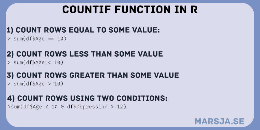
countif function in R
Countif function in R

Next, we will introduce the dplyr package, which provides a more intuitive syntax for data manipulation. We will show you how to use the mutate() and sum() functions in dplyr to achieve the same result as the sum() function many times.

Finally, we will create a custom countif function that combines the power of base R and dplyr. Our custom function will allow you to easily count the number of rows in a data frame that meet a specific condition, using a simple and intuitive syntax.

By the end of this blog post, you will have a deep understanding of how to use the countif function in R to analyze and manipulate data frames in cognitive hearing science.

Read more

How to do a Kruskal-Wallis Test in R

Kruskal-Wallis R

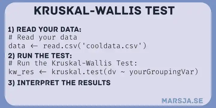
This post will teach you how to carry out the Kruskal-Wallis test in R. The Kruskal-Wallis test is a non-parametric statistical test used to determine whether there is a significant difference in the median values of two or more independent groups. This method is used when the analyzed data is not normally distributed, or the sample size is small. In addition, when the normality assumption is violated, the Kruskal-Wallis test is used instead of the traditional one-way analysis of variance (ANOVA).

3 steps to the kruskal wallis test in R

Read more

How to Extract Year from Date in R with Examples

In this tutorial, you will learn how to extract year from date in R. You will learn by a couple of examples containing R code along with a description of the code. To know how to extract the year from DateTime may be needed when working with data containing datetime (e.g., 2020-08-24 10:34:00) and you want to do e.g. time series analysis but only want to use year.

how to get year from date in R

As you may already know, R is a versatile statistical programming environment, and there are many ways to extract elements, such as year, from datetime.  For example, we can separate year using the format() function. In this post, however, we need to start by converting a vector, or a column in a dataframe (e.g., to a POSIXct class) as well as use the lubridate package. It is, of course, possible to adapt the examples in this post to extract time, and to extract day.

Read more

How to Read and Write Stata (.dta) Files in R with Haven

reading & writing stata files in R

In this post, we will learn how to read Stata (.dta) files in R statistical environment. Specifically, we will learn 1) how to read .dta files in R using Haven, and 2) how to write dataframes to .dta file.

Data Import in R: Reading Stata Files

R is, as we all know, a superb statistical programming environment. When importing and storing data, we can store it in the native .rda format. However, if we have a collaborator that uses other statistical software (e.g., Stata) and/or that are storing their data in different formats (e.g., .dta files).

Now, this is when R shows us its brilliance; as an R user, we can load data from a range of file formats; e.g., SAS (.7bdat), Stata (.dta), Excel (e.g., .xlsx), and CSV (.csv). On this site, there are other tutorials on how to import data from (some) of these formats:

Before we go on and learn how to read Stata files in R, we will answer the questions:

Read more

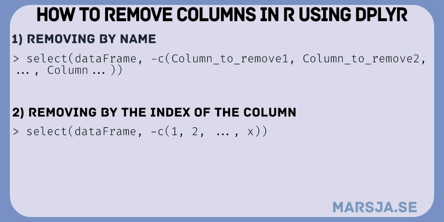
How to Remove a Column in R using dplyr (by name and index)

delete a column in R

In this blog post, we will explore an important skill in data manipulation: how to efficiently remove a column in R. Whether you are analyzing psychological data, studying the effects of noise exposure in hearing science, or working with large datasets in data science, there are often scenarios where you need to remove unnecessary variables. By mastering the technique of removing columns, you can streamline your data analysis process, enhance data clarity, and improve computational efficiency.

When working with psychological data, you may have collected numerous variables during your study, including demographic information, survey responses, and experimental measures. To focus on specific research questions or simplify your analysis, removing irrelevant columns is crucial. Similarly, in the field of hearing science, you may gather a wide range of auditory measurements, but only a subset might be relevant to your investigation. By removing unnecessary columns, you can narrow down your data to the key variables of interest.

how do remove columns in r
remove columns in R with dplyr

In data science, working with large datasets is quite common. Large datasets often contain numerous columns, and handling unnecessary or redundant variables can significantly impact computational efficiency. Removing extraneous columns helps reduce memory usage and accelerates data processing, allowing you to concentrate on the essential aspects of your analysis.

In the following sections, we will learn various techniques we can use to remove columns in R, including using base R functions and leveraging popular packages like dplyr. We will explore practical examples and provide step-by-step instructions to equip you with the necessary skills to confidently remove columns from your datasets. So, let us dive in and master the art of removing columns in R!

Read more

How to Calculate Descriptive Statistics in R the Easy Way with dplyr

descriptive statistics in R

In this tutorial, you will learn how to calculate descriptive statistics in R, a fundamental tool for data analysis. Descriptive statistics provide an overview of the key characteristics of a dataset, including measures of central tendency, variability, and distribution. These statistics help us to understand the distribution of data and can be used to identify patterns and relationships within the data.

Outline

We will start by installing the necessary R-packages and importing data. Then, we will explore how to calculate measures of central tendency, such as the mean and median, and how to calculate them by one or two groups. We will also cover less commonly used measures of central tendency, such as geometric, harmonic, and trimmed mean.

Next, we will dive into measures of variability, including the standard deviation, interquartile range, and quantiles. These measures help us understand the data’s spread and can be used to identify outliers or unusual observations.

We will also explore how to use the psych and dplyr packages to calculate summary and descriptive statistics by group. Additionally, we will learn how to create a LaTeX table with descriptive statistics and how to save descriptive statistics to a CSV file for future analysis.

By the end of this tutorial, you will have a solid understanding of using R to calculate and interpret descriptive statistics. Whether new to R or looking to expand your data analysis skills, this tutorial will provide the knowledge and tools needed to work confidently with descriptive statistics in R.

Note, in a recent post, you learn how to quickly explore your data with one of Tukey’s exploratory data analysis methods:

Why Descriptive Statistics?

Calculating descriptive statistics in R is crucial in any data analysis process. Descriptive statistics provide a concise summary of a dataset’s key characteristics, helping us understand its distribution and identify patterns and relationships within the data.

Read more

How to Read & Write SPSS Files (.sav) in R Statistical Environment

import .sav into R

In data analysis, it is common to encounter data saved in different formats, and being able to read them is crucial. In this blog post, we will focus on reading .sav files in R. These files are created by SPSS, a popular software used for statistical analysis. There are several ways to read .sav files in R, including using the read_sav function from the haven package or the read.spss function from the foreign package. We’ll cover both methods in this post, along with tips on importing data from URLs and converting R dataframes to SPSS files. Additionally, we will explore how to import data from other common formats like CSV and Excel to SPSS files. By the end of this post, you will understand how to read and write SPSS files in R and be ready to tackle any data import challenges you might face in your analysis.

Read more

How to Import Data: Reading SAS Files in R with Haven & sas7dbat

In this post, we are going to learn how to read a SAS (. sas7bdat) file in R. More specifically, we are going to use the packages haven, and sas7bdat. Furthermore, we will also learn how to load .sas7bdat files into R using RStudio.

If you are interested in other methods on how to import data in R:

Read more

How to Use Binder and R for Reproducible Research

In a previous post, we learned how to use Binder and Python for reproducible research. Now, we are going to learn how to create a Binder for our data analysis in R, so it can be fully reproduced by other researchers. More specifically, in this post, we will learn how to use Binder for reproducible research.

Many researchers upload their code for data analysis and visualization using git (e.g., GitHub, Gitlab).

No doubt, uploading your R scripts is great. However, we also need to make sure that we share the complete computational environment so that our code can be re-run and so that others can reproduce the results. That is, to make sure that other researchers really can reproduce our code, we need a way to capture the versions of the R packages we used when publishing our research.

Read more