This post will cover how to do a Multivariate Analysis of Variance (MANOVA) in R! In our previous posts, we have covered topics like probit regression and correlation, disentangling the layers of statistical analysis in R. Today, we are taking a closer look at MANOVA, a powerful extension of Analysis of Variance (ANOVA) that becomes indispensable when dealing with multiple dependent variables.
Understanding group differences on a single dependent variable is crucial in statistical analysis. However, situations arise where we seek insights across several dependent variables simultaneously. The traditional approach might involve multiple ANOVA tests, one for each dependent variable. However, this method introduces the risk of inflating the family-wise error rate, increasing the likelihood of Type I errors.
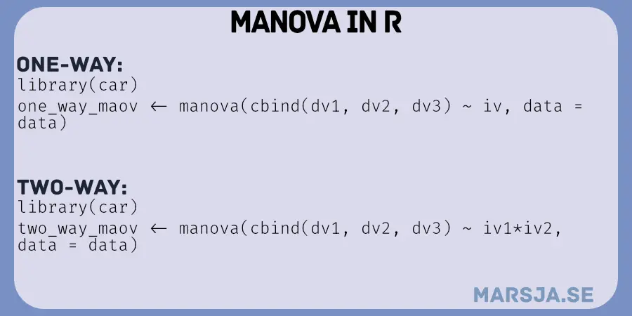
Enter MANOVA, which is designed to address precisely this challenge. Standing for Multivariate Analysis of Variance, MANOVA extends the principles of ANOVA to scenarios with two or more dependent variables. In this blog post, we will guide you through performing one-way and two-way MANOVA in R, interpreting and visualizing the results.
Table of Contents
- Outline
- Prerequisites
- Understanding MANOVA
- Illustrating MANOVA in Context
- Synthetic Data
- One-Way MANOVA in R
- How to Interpret One-Way MANOVA Results in R
- How to Visualize MANOVA in R
- Two-Way MANOVA in R
- How to Interpret Two-Way MANOVA Results in R
- Conclusion
Outline
The outline of this post is as follows. First, we learn about MANOVA, focusing on its foundational principles. We learn about the hypotheses (H1 and H0) that underscore MANOVA’s analytical framework and explore the critical assumptions integral to its application. Following this, we illustrate the practical application of MANOVA in a contextual setting, providing an view of its real-world implications.
Moving forward, we engage in a hands-on demonstration using synthetic data, offering a step-by-step guide to conducting one-way MANOVA in R. We navigate through the intricacies of interpreting one-way MANOVA results, emphasizing the significance of these statistical insights.
Our exploration extends to the data visualization, where we learn how to effectively present MANOVA results using graphical representations in R. Subsequently, we broaden our analytical toolkit, tackling the complexities of two-way MANOVA in R. With a focus on practical examples, we elucidate the nuanced interpretation of results when dealing with multiple independent variables.
The post concludes with a summary, highlighting key takeaways and emphasizing the importance of mastering MANOVA for robust statistical analysis.
Prerequisites
Prerequisites for this tutorial include a basic understanding of R. If you plan to use ggplot2 and tidyr for visualization, ensure they are installed by using the commands install.packages("ggplot2") and install.packages("tidyr"). Additionally, having an updated version of R is advisable for compatibility and enhanced features. Check your R version using sessionInfo(), and update R with installr::updateR() if needed. Familiarity with fundamental statistical concepts such as p-values is recommended to grasp MANOVA interpretation comprehensively.
Understanding MANOVA
First, we will have a quick look at what MANOVA is. MANOVA is an acronym that stands for Multivariate Analysis of Variance. In data analysis, situations often arise where multiple response variables, also known as dependent variables, come into play. MANOVA is an powerful tool by allowing us to collectively test these variables.
The null hypothesis (H0) for a MANOVA states no significant differences in the dependent variables’ mean vectors across the independent variable(s) levels. In other words, it asserts that the independent variable(s) have no overall effects on the dependent variables.
On the other hand, the alternative hypothesis (H1 or Ha) posits significant differences in at least one of the dependent variables across the levels of the independent variable(s). This implies that the mean vectors of the dependent variables are not equal across groups.
In mathematical terms, the null hypothesis can be expressed as:
- H0: μ1 = μ2 = … = μk (where μ represents the mean vector for each group)
And the alternative hypothesis as:
- Ha: At least one μi is different (where i refers to the groups being compared)
Assumptions
In Multivariate Analysis of Variance (MANOVA), it is important to be aware of certain assumptions to ensure the reliability of results. First and foremost, the assumption of multivariate normality is important, implying that the residuals should ideally follow a normal distribution. We can assess this assumption through tests of normality of residuals in R. Additionally, homogeneity of covariance matrices across groups is assumed, emphasizing the need for equality in variances among groups. Lastly, linearity and independence of observations are essential assumptions, underlining the importance of a comprehensive understanding of data characteristics before delving into MANOVA analyses.
Illustrating MANOVA in Context
Before getting into the mechanics of conducting MANOVA in R, let us look at a practical example where this statistical method can be usable. Imagine a scenario where we hypothesize that a novel therapy surpasses the effectiveness of a more conventional approach or multiple therapies. This hypothesis gains significance in cognitive psychology, particularly among hearing-impaired individuals.
Consider exploring the impact of different therapies (independent variable) on various aspects of well-being. Picture our interest in understanding not just the therapeutic effects on a specific psychological disorder, such as depression, but also the concurrent influence on life satisfaction, mitigation of suicide risk, and other pertinent factors. MANOVA becomes useful, enabling the simultaneous testing of hypotheses across all three dependent variables, providing a comprehensive understanding of the therapeutic landscape for hearing-impaired individuals.
Synthetic Data
Here is a synthetic dataset we will use to practice two-way and one-way MANOVA using R:
# Set seed for reproducibility
set.seed(123)

# Generate data for Hearing Status (categorical: normal or impaired)
hearing_status <- sample(c("Normal", "Impaired"), 100, replace = TRUE)

# Generate data for Gender (categorical: male or female)
gender <- sample(c("Male", "Female"), 100, replace = TRUE)

# Generate dependent variables
# Assume Hearing Test Scores, Memory Performance, and Reaction Time as dependent variables
hearing_test_scores <- rnorm(100, mean = ifelse(hearing_status == "Normal", 75, 60), sd = 10)
memory_performance <- rnorm(100, mean = ifelse(hearing_status == "Normal", 80, 65), sd = 12)
reaction_time <- rnorm(100, mean = ifelse(hearing_status == "Normal", 0.5, 0.7), sd = 0.1)

# Create a data frame
data <- data.frame(
  Hearing_Status = as.factor(hearing_status),
  Gender = as.factor(gender),
  Hearing_Test_Scores = hearing_test_scores,
  Memory_Performance = memory_performance,
  Reaction_Time = reaction_time
)Code language: R (r)
In the code chunk above, we set the seed for reproducibility using set.seed(123). We then generated synthetic data for a simulated study on hearing-impaired individuals. Two categorical independent variables, Hearing_Status and Gender, were created, with ‘Normal’ and ‘Impaired’ for hearing status and ‘Male’ and ‘Female’ for gender. Next, we created three dependent variables. These represent Hearing Test Scores, Memory Performance, and Reaction Time. Finally, we organized the data into a dataframe named ‘data’ for subsequent analysis.
One-Way MANOVA in R
To perform a one-way MANOVA in R on the simulated dataset, we can use the following code:
# Load necessary library for MANOVA
library(car)

# One-way MANOVA
one_way_manova <- manova(cbind(Hearing_Test_Scores, Memory_Performance, Reaction_Time) ~ Hearing_Status, data = data)

# Display the summary of the one-way MANOVA
summary(one_way_manova)
Code language: PHP (php)
In the code chunk above, we begin by loading the essential car library, a toolkit that proves instrumental in conducting advanced statistical analyses. Subsequently, we execute a one-way MANOVA. We used the simulated dataset to test the influence of ‘Hearing Status’ on the dependent variables. The dependent variables include ‘Hearing Test Scores,’ ‘Memory Performance,’ and ‘Reaction Time.’ The manova function efficiently accommodates multiple dependent variables, and in this case, it assesses the statistical significance of differences in mean vectors across various levels of ‘Hearing Status.’ Following the execution of the one-way MANOVA, the summary function provides a comprehensive overview of the results. This summary includes statistical metrics such as Wilks’ Lambda, Pillai’s Trace, Hotelling-Lawley Trace, and Roy’s Largest Root, offering insights into the overall significance of ‘Hearing Status’ on the combined set of dependent variables. In the next section, we will learn how to interpret the results from the MANOVA.
How to Interpret One-Way MANOVA Results in R
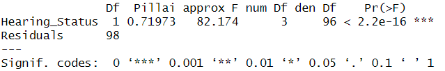
We can use the output from the summary() function to interpret the MANOVA results in R. First, we look at the ‘Hearing_Status’ row. The Pillai’s Trace statistic, which measures the proportion of variance explained, is 0.71973. This suggests a substantial effect of ‘Hearing_Status’ on the combined dependent variables. The approximate F-statistic of 82.174, with 1 and 98 degrees of freedom, indicates a highly significant result (p < 2.2e-16). The interpretation is that at least one mean vector of the dependent variables differs significantly across the levels of ‘Hearing_Status.’ The residuals, representing unexplained variance, have 98 degrees of freedom. In summary, the MANOVA results strongly support the hypothesis that ‘Hearing_Status’ significantly influences the joint variation in ‘Hearing Test Scores,’ ‘Memory Performance,’ and ‘Reaction Time,’ providing valuable insights into our dataset’s cognitive and reaction time metrics.
How to Visualize MANOVA in R
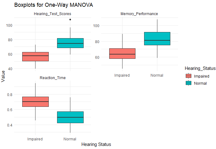
Visualizing the outcomes of a one-way MANOVA in R can be effectively accomplished through diverse graphical methods. A commonly employed technique is leveraging box plots, which depict group differences and the distribution of individual variables. Box plots are particularly insightful for understanding the spread of data within each group and identifying potential variations among categories.
Here is an example illustrating how to generate box plots for a one-way MANOVA in R:
# Load necessary libraries
library(ggplot2)
library(tidyr)

# Create boxplots using ggplot2 and pivot_longer
data_long <- pivot_longer(data, cols = -c(Hearing_Status, Gender), names_to = "Variable", values_to = "Value")

ggplot(data_long, aes(x = Hearing_Status, y = Value, fill = Hearing_Status)) +
  geom_boxplot() +
  facet_wrap(Variable ~ ., scales = "free_y", ncol = 2) +
  labs(title = "Boxplots for One-Way MANOVA",
       x = "Hearing Status",
       y = "Value") +
  theme_minimal()Code language: R (r)
In the code chunk above, we loaded the necessary libraries, specifically ‘ggplot2’ and ‘tidyr’. Next, we used the ‘pivot_longer’ function to transform the data from a wide to long in R, facilitating its compatibility with ‘ggplot2.’ This step is essential for creating boxplots that visualize the distribution of multiple dependent variables across different independent variable levels. The resulting boxplots, generated using ‘ggplot2,’ clearly represent the one-way MANOVA results, showcasing variations in ‘Hearing Status’ for each dependent variable. We used ‘facet_wrap’ to organize the boxplots efficiently, allowing for easy comparison. Here is the resulting plot:
Two-Way MANOVA in R
Here is to do a two-way MANOVA in R:
# Two-way MANOVA
two_way_manova <- manova(cbind(Hearing_Test_Scores, Memory_Performance, Reaction_Time) ~ Hearing_Status * Gender, data = data)
summary(two_way_manova)Code language: HTML, XML (xml)
In the code chunk above, we extended our analysis from the previous one-way MANOVA to a two-way MANOVA. Notably, we introduced an interaction term between ‘Hearing_Status’ and ‘Gender’ in the model formula. This alteration enables us to assess not only the main effects of ‘Hearing_Status’ and ‘Gender’ but also their combined influence on the dependent variables. Using the manova function, we comprehensively examine the multivariate differences in ‘Hearing Test Scores,’ ‘Memory Performance,’ and ‘Reaction Time.’ The subsequent summary output provides detailed insights into the statistical significance of these effects, empowering a nuanced interpretation of the interplay between hearing status, gender, and cognitive metrics.
How to Interpret Two-Way MANOVA Results in R
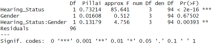
In the two-way MANOVA results above, we observe significant multivariate effects. ‘Hearing_Status’ exhibits a substantial impact (Pillai’s Trace = 0.73214, F = 85.641, p < 2e-16), indicating differences in cognitive metrics based on hearing status. However, ‘Gender’ alone does not significantly influence the dependent variables (Pillai’s Trace = 0.01608, F = 0.512, p = 0.67502). Notably, the interaction effect ‘Hearing_Status:Gender’ is statistically significant (Pillai’s Trace = 0.13179, F = 4.756, p = 0.00393), suggesting that the joint influence of hearing status and gender contributes to variations in the cognitive measures. These results underscore the importance of considering the combined effects of ‘Hearing_Status’ and ‘Gender’ when interpreting the observed differences in ‘Hearing Test Scores,’ ‘Memory Performance,’ and ‘Reaction Time.’
Conclusion
This comprehensive tutorial taught us how to conduct MANOVA. First, we laid the foundation, exploring the hypotheses underlying MANOVA and highlighting its essential assumptions. Next, we continued with a hands-on demonstration using synthetic data, elucidating the step-by-step process of conducting one-way MANOVA in R. The subsequent sections unveiled key insights on interpreting MANOVA results obtained with R.
Next, we learned to do a two-way MANOVA, examining interactions between multiple independent variables. We also learned how to interpret two-way MANOVA results, recognizing the significance of joint effects on the observed multivariate differences.
Remember the assumptions of multivariate normality, homogeneity of covariance matrices, linearity, and independence. Make use of visualizations like box plots to gain nuanced insights. If you have questions or suggestions, share your thoughts in the comments below. Remember to share this post with your peers, fostering a collaborative learning environment.