Two-way repeated measures ANOVA in Python can be used to analyze experiments with two within-subject factors. If you are new to repeated measures ANOVA, you may first want to read my tutorials on within-subjects designs using rpy2 (i.e., R from within Python) and repeated measures ANOVA using Pyvttbll. In this tutorial, we will extend the previous examples to a two-way repeated measures ANOVA using pyvttbl. Although the example focuses on a two-factor design, the same approach can be applied to more complex repeated-measures designs.
We will begin by importing the required Python packages:
import numpy as np
import pyvttbl as pt
from collections import namedtupleCode language: Python (python)
We will use NumPy to simulate a repeated-measures dataset with two within-subject factors. The first factor (iv1) has two levels, and the second (iv2) has three levels. As in many of my examples, the dependent variable is response time (rt). To keep the example simple, the population means are defined in the values variable.
Table of Contents
- Simulate data
- Two-way ANOVA for within-subjects design in Python
- Output ANOVA table
- Alternative Data Analysis Techniques
Simulate data
Here is an example data we can use for the practice.
N = 20
P = [1,2]
Q = [1,2,3]

values = [[998,511], [1119,620], [1300,790]]

sub_id = [i+1 for i in xrange(N)]*(len(P)*len(Q))
mus = np.concatenate([np.repeat(value, N) for value in values]).tolist()
rt = np.random.normal(mus, scale=112.0, size=N*len(P)*len(Q)).tolist()
iv1 = np.concatenate([np.array([p]*N) for p in P]*len(Q)).tolist()
iv2 = np.concatenate([np.array([q]*(N*len(P))) for q in Q]).tolist()


Sub = namedtuple('Sub', ['Sub_id', 'rt','iv1', 'iv2'])
df = pt.DataFrame()

for idx in xrange(len(sub_id)):
    df.insert(Sub(sub_id[idx],rt[idx], iv1[idx],iv2[idx])._asdict())Code language: Python (python)
Before running the analysis, it is a good idea to inspect the data visually. pyvttbl includes a box_plot() method that can be used to create boxplots for each combination of the two factors:
df.box_plot('rt', factors=['iv1', 'iv2'])Code language: Python (python)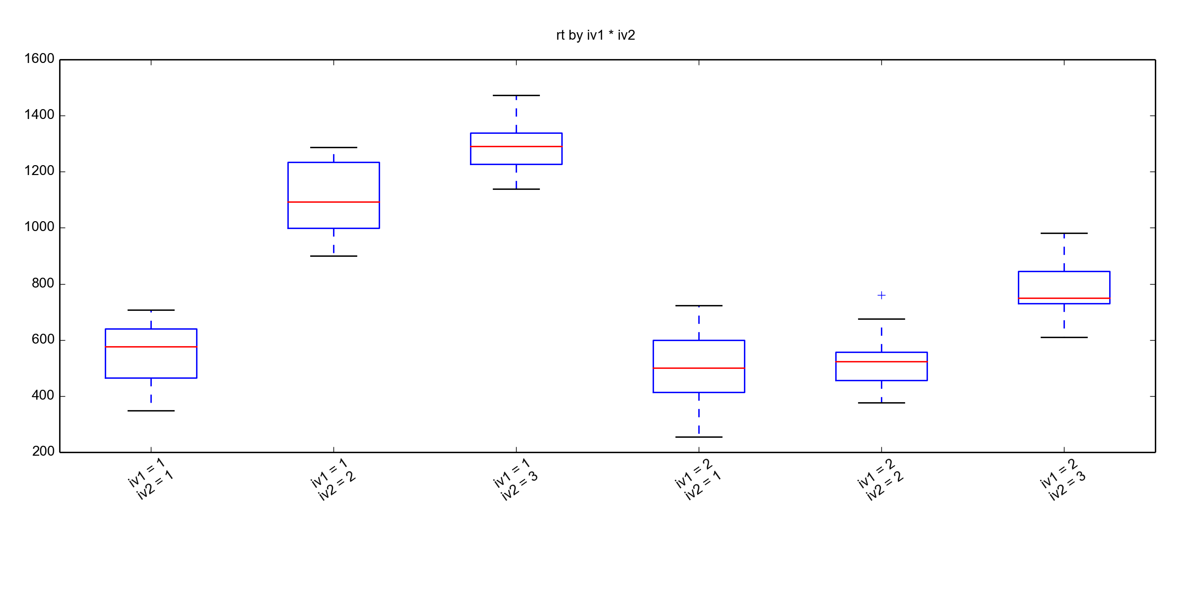
Two-way ANOVA for within-subjects design in Python
Running a two-way repeated measures ANOVA with pyvttbl only requires a single call to the anova() method. Specify the dependent variable, the participant identifier (sub), and the within-subject factors (wfactors):
aov = df.anova('rt', sub='Sub_id', wfactors=['iv1', 'iv2'])
print(aov)Code language: Python (python)
If you are interested in between-subjects designs, see my tutorials on one-way ANOVA for independent measures and two-way ANOVA for independent measures. pyvttbl also supports mixed (split-plot) ANOVA by adding the bfactors argument for the between-subject factor(s).
Running the analysis returns a complete ANOVA table containing the F statistic, p values, mean squares, effect sizes (generalized eta squared), confidence intervals, and results for the interaction between the two within-subject factors. The output also includes corrections for violations of sphericity, such as the Greenhouse-Geisser correction. The full output is shown at the end of this tutorial. Since the default formatting is not particularly easy to read, I also include a helper function later in the post to extract the most commonly reported statistics.
Update (2017-07-03): If your installed version of NumPy is greater than 1.11.x, you will run into a Float and NoneType error. One quick solution is to downgrade NumPy to 1.11.x. I created a post, Step-by-step guide for solving the Pyvttbl Float and NoneType error, in which I show how to install NumPy 1.11.x in a virtual environment. This way, you can run your ANOVAs without having to uninstall NumPy.
Output ANOVA table
Here is the output table we get:
rt ~ iv1 * iv2

TESTS OF WITHIN SUBJECTS EFFECTS

Measure: rt
  Source                            Type III      eps      df         MS           F        Sig.      et2_G   Obs.     SE     95% CI    lambda    Obs.
                                       SS                                                                                                         Power
=======================================================================================================================================================
iv1           Sphericity Assumed   4419957.211       -        1   4419957.211   324.248   2.128e-13   3.295     60   16.096   31.548   1023.941       1
              Greenhouse-Geisser   4419957.211       1        1   4419957.211   324.248   2.128e-13   3.295     60   16.096   31.548   1023.941       1
              Huynh-Feldt          4419957.211       1        1   4419957.211   324.248   2.128e-13   3.295     60   16.096   31.548   1023.941       1
              Box                  4419957.211       1        1   4419957.211   324.248   2.128e-13   3.295     60   16.096   31.548   1023.941       1
-------------------------------------------------------------------------------------------------------------------------------------------------------
Error(iv1)    Sphericity Assumed    258996.722       -       19     13631.406
              Greenhouse-Geisser    258996.722       1       19     13631.406
              Huynh-Feldt           258996.722       1       19     13631.406
              Box                   258996.722       1       19     13631.406
-------------------------------------------------------------------------------------------------------------------------------------------------------
iv2           Sphericity Assumed   5257766.564       -        2   2628883.282   206.008   4.023e-21   3.920     40   18.448   36.158    433.701       1
              Greenhouse-Geisser   5257766.564   0.550    1.101   4777252.692   206.008   1.320e-12   3.920     40   18.448   36.158    433.701       1
              Huynh-Feldt          5257766.564   0.550    1.101   4777252.692   206.008   1.320e-12   3.920     40   18.448   36.158    433.701       1
              Box                  5257766.564   0.500        1   5257766.564   206.008   1.192e-11   3.920     40   18.448   36.158    433.701       1
-------------------------------------------------------------------------------------------------------------------------------------------------------
Error(iv2)    Sphericity Assumed    484921.251       -       38     12761.086
              Greenhouse-Geisser    484921.251   0.550   20.911     23189.668
              Huynh-Feldt           484921.251   0.550   20.911     23189.668
              Box                   484921.251   0.500       19     25522.171
-------------------------------------------------------------------------------------------------------------------------------------------------------
iv1 *         Sphericity Assumed   1622027.598       -        2    811013.799    83.220   1.304e-14   1.209     20   22.799   44.687     87.600   1.000
iv2           Greenhouse-Geisser   1622027.598   0.545    1.091   1486817.582    83.220   6.085e-09   1.209     20   22.799   44.687     87.600   1.000
              Huynh-Feldt          1622027.598   0.545    1.091   1486817.582    83.220   6.085e-09   1.209     20   22.799   44.687     87.600   1.000
              Box                  1622027.598   0.500        1   1622027.598    83.220   2.262e-08   1.209     20   22.799   44.687     87.600   1.000
-------------------------------------------------------------------------------------------------------------------------------------------------------
Error(iv1 *   Sphericity Assumed    370327.311       -       38      9745.456
iv2)          Greenhouse-Geisser    370327.311   0.545   20.728     17866.175
              Huynh-Feldt           370327.311   0.545   20.728     17866.175
              Box                   370327.311   0.500       19     19490.911

TABLES OF ESTIMATED MARGINAL MEANS

Estimated Marginal Means for iv1
iv1    Mean     Std. Error   95% Lower Bound   95% Upper Bound
==============================================================
1     983.755       43.162           899.157          1068.354
2     599.917       21.432           557.909           641.925

Estimated Marginal Means for iv2
iv2     Mean     Std. Error   95% Lower Bound   95% Upper Bound
===============================================================
1      525.025       19.324           487.150           562.899
2      814.197       49.416           717.342           911.053
3     1036.286       43.789           950.459          1122.114

Estimated Marginal Means for iv1 * iv2
iv1   iv2     Mean     Std. Error   95% Lower Bound   95% Upper Bound
=====================================================================
1     1      553.522       24.212           506.066           600.978
1     2     1103.488       28.411          1047.804          1159.173
1     3     1294.256       19.773          1255.501          1333.011
2     1      496.528       29.346           439.009           554.047
2     2      524.906       20.207           485.301           564.512
2     3      778.317       21.815           735.560           821.073
Alternative Data Analysis Techniques
In this section, you will find some blog posts that cover other data analysis techniques:
- How to Perform a Two-Sample T-test with Python: 3 Different Methods
- Probabilistic Programming in Python
- How to Perform Mann-Whitney U Test in Python with Scipy and Pingouin
Hi there. Thanks for your excellent blog. I’m trying to run a two-way repeated mesures ANOVA using pyvttbl as you explain. I use python 2.7 and installed pyvttbl via pip. I was able to import pyvttbl and create the dataframe just fine. However, when I run the test, I get this error: TypeError: unsupported operand type(s) for +: ‘float’ and ‘NoneType’. Can you help? Thanks in advance!
Hey Veronica,
Have you solved the problem? When I wrote this blog, this did not happen. However, I tried to run the script again and get the same problem. I am not sure what is going on here but I will try to find out given that you did not solve it.
Please let me know if and how you solved the problem.
Erik
Hi,
I’ve had the same error but by googling it, I found a similar issue with the library py-faster-rcnn (https://github.com/rbgirshick/py-faster-rcnn/issues/481#issuecomment-278709605). You have to uninstall the current version of numpy and install numpy v1.11.0. For me, it works !
Damien
Thanks for leaving your comment here, Damien!
I will update the posts later and reference to your solution.
Erik
Hi Erik,
I met the same problem when I ran my analysis. In my study, the design is a 2x3x3 repeated measure ANOVA. And my code is straightforward, import pyvttbl as pt
df = pt.DataFrame()
df.read_tbl(‘Z_score_filtered.csv’)
aov = df.anova(‘Z_score’, sub=’ID’, wfactors=[‘Task_types’, ‘conditions’, ‘Question’])
print(aov)
But it returned the error “unsupported operand type(s) for +: ‘float’ and ‘NoneType'”. I have checked my data file and found Z_score was stored as numpy.float64. Is it the reason I have this error message? Should I change my data from numpy.float64 to long or other data type?
Thanks for your help!
Hey Shengjie,
Right now I don’t have a solution for this problem other than the one Damien gave here in the comments. It seems like you have to have Python 1.11.0 (maybe other versions work to but it worked for Damien). Hope it helps. I will update my post(s) with this solution. I don’t think Pyvttbl have been updated for 4 years, or so. Maybe someone should build a new package/update Pyvttbl. 🙂