Three ways to do a two-way ANOVA with Python

Two-way ANOVA in Python allows you to test the effects of two categorical factors simultaneously and assess whether they interact. If you are new to analysis of variance, you may want to start with my tutorial on One-Way ANOVA in Python or browse the other guides in my Python Data Analysis Tutorials.

In this tutorial, we will calculate a two-way ANOVA in several different ways. We will first work through the calculations behind the ANOVA table, then perform the analysis using statsmodels, pyvttbl, and Pingouin.

Compared with a one-way ANOVA, a two-way ANOVA can provide a more efficient design because it accounts for variation associated with two factors instead of one. More importantly, it allows you to test whether the effect of one factor depends on the level of the other by including an interaction term.

Throughout this tutorial, we will use an experiment with two factors (supp and dose) as an example. As with one-way ANOVA, observations should be independent, and the design is typically balanced when the analysis is performed using the manual calculations presented below.

We discussed linear models earlier – and ANOVA is indeed a kind of linear model – the difference being that ANOVA is where you have discrete factors whose effect on a continuous (variable) result you want to understand. Make sure to check the recent posts about how to perform two-sample t-test in Python and Mann-Whitney U-test in Python.

Table of Contents

• Python 2-way ANOVA
  • Calculation of Sum of Squares
    • Degrees of Freedom
    • Sum of Squares
      • Sum of Squares A – supp
      • Sum of Squares B – dose
      • Sum of Squares Total
      • Sum of Squares Within (error/residual)
      • Sum of Squares interaction
    • Mean Squares
      • Mean Square A
      • Mean Square B
      • Mean Square AxB
      • Mean Square Within/Error/Residual
    • F-ratio
    • Obtaining p-values
    • Output ANOVA table
  • Two-way ANOVA using Statsmodels
    • Output ANOVA table
  • Two-way ANOVA in Python using pyvttbl
  • Measure: len
• Two-Way ANOVA using Pingouin (Bonus)

Python 2-way ANOVA

First of all, we need to import all the tools needed to carry out the ANOVA:

import pandas as pdimport statsmodels.api as sm
from statsmodels.formula.api import ols
from statsmodels.stats.anova import anova_lm
from statsmodels.graphics.factorplots import interaction_plot
import matplotlib.pyplot as plt
from scipy import statsCode language: Python (python)

In the code above, we import all the necessary Python libraries and methods to implement the first two methods in Python (calculation and Statsmodels). In the last, and third, method for doing Python ANOVA, we are going to use Pyvttbl. As in the previous post on one-way ANOVA using Python, we will use a set of data that is available in R but can be downloaded here: TootGrowth Data. Pandas is used to create a dataframe that is easy to manipulate.

datafile = "ToothGrowth.csv"
data = pd.read_csv(datafile)Code language: Python (python)

It can be helpful to explore the data before proceeding with inferential statistics. statsmodels has methods for visualizing factorial data. We are going to use the method interaction_plot.

fig = interaction_plot(data.dose, data.supp, data.len,
             colors=['red','blue'], markers=['D','^'], ms=10)Code language: Python (python)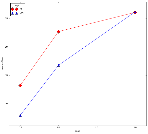

• Save

Calculation of Sum of Squares

Calculating the sum of squares (the variance in the data) is quite simple in Python. First, we determine the sample size (N) and the degrees of freedom required. We will use them later to calculate the mean square. Once we have the degrees of freedom, we proceed to calculate the sum of squares.

Degrees of Freedom

N = len(data.len)
df_a = len(data.supp.unique()) - 1
df_b = len(data.dose.unique()) - 1
df_axb = df_a*df_b 
df_w = N - (len(data.supp.unique())*len(data.dose.unique()))Code language: Python (python)

Sum of Squares

• Save

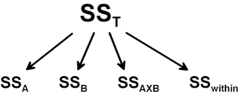
To calculate the sums of squares for A, B, and Total, we need the grand mean. Using the Pandas DataFrame method mean on the dependent variable only will give us the grand mean:

grand_mean = data['len'].mean()Code language: Python (python)

The grand mean is simply the mean of all scores of len.

Sum of Squares A – supp

We start with the calculation of Sum of Squares for the factor A (supp).

ssq_a = sum([(data[data.supp ==l].len.mean()-grand_mean)**2 for l in data.supp])Code language: Python (python)

Sum of Squares B – dose

Calculation of the second Sum of Squares, B (dose), is pretty much the same but over the levels of that factor.

ssq_b = sum([(data[data.dose ==l].len.mean()-grand_mean)**2 for l in data.dose])<Code language: Python (python)

Sum of Squares Total

ssq_t = sum((data.len - grand_mean)**2)Code language: Python (python)

Sum of Squares Within (error/residual)

Next, we need to calculate the Sum of Squares Within, which is sometimes referred to as error or residual.

vc = data[data.supp == 'VC']
oj = data[data.supp == 'OJ']
vc_dose_means = [vc[vc.dose == d].len.mean() for d in vc.dose]
oj_dose_means = [oj[oj.dose == d].len.mean() for d in oj.dose]
ssq_w = sum((oj.len - oj_dose_means)**2) +sum((vc.len - vc_dose_means)**2Code language: Python (python)

Sum of Squares interaction

Since we have a two-way design, we need to calculate the Sum of Squares for the interaction of A and B.

ssq_axb = ssq_t-ssq_a-ssq_b-ssq_wCode language: Python (python)

Mean Squares

We continue with the calculation of the mean square for each factor, the interaction of the factors, and within.

Mean Square A

ms_a = ssq_a/df_aCode language: Python (python)

Mean Square B

ms_b = ssq_b/df_bCode language: Python (python)

Mean Square AxB

ms_axb = ssq_axb/df_axbCode language: Python (python)

Mean Square Within/Error/Residual

ms_w = ssq_w/df_wCode language: Python (python)

F-ratio

The F-statistic is simply the mean square for each effect and the interaction divided by the mean square for within (error/residual).

f_a = ms_a/ms_w
f_b = ms_b/ms_w
f_axb = ms_axb/ms_wCode language: Python (python)

Obtaining p-values

We can use the scipy.stats method f.sf to check whether our obtained F-ratios exceed the critical value. To do that, we need to use our F-values for each effect and interaction, as well as their degrees of freedom and the degrees of freedom within.

p_a = stats.f.sf(f_a, df_a, df_w)
p_b = stats.f.sf(f_b, df_b, df_w)
p_axb = stats.f.sf(f_axb, df_axb, df_w)Code language: Python (python)

The results are currently stored in many variables. To obtain a more readable result, we can create a DataFrame that will contain our ANOVA table.

results = {'sum_sq':[ssq_a, ssq_b, ssq_axb, ssq_w],
           'df':[df_a, df_b, df_axb, df_w],
           'F':[f_a, f_b, f_axb, 'NaN'],
            'PR(>F)':[p_a, p_b, p_axb, 'NaN']}
columns=['sum_sq', 'df', 'F', 'PR(>F)']
aov_table1 = pd.DataFrame(results, columns=columns,
                          index=['supp', 'dose', 
                          'supp:dose', 'Residual'])Code language: Python (python)

As a Psychologist, most of the journals we publish in require us to report effect sizes. Common software, such as SPSS, has eta squared as output. However, eta squared is an overestimation of the effect. To obtain a less biased measure of effect size, we can use omega squared. The following two functions add eta squared and omega squared to the above DataFrame that contains the ANOVA table.

def eta_squared(aov):
    aov['eta_sq'] = 'NaN'
    aov['eta_sq'] = aov[:-1]['sum_sq']/sum(aov['sum_sq'])
    return aov
def omega_squared(aov):
    mse = aov['sum_sq'][-1]/aov['df'][-1]
    aov['omega_sq'] = 'NaN'
    aov['omega_sq'] = (aov[:-1]['sum_sq']-(aov[:-1]['df']*mse))/(sum(aov['sum_sq'])+mse)
    return aov
eta_squared(aov_table1)
omega_squared(aov_table1)
print(aov_table1)Code language: Python (python)

Output ANOVA table

• Save

• Jupyter Notebook containing the code above

Two-way ANOVA using Statsmodels

There is, of course, a much easier way to do Two-way ANOVA with Python. We can use Statsmodels, which has a similar model notation as many R packages (e.g., lm). We start with the formulation of the model:

formula = 'len ~ C(supp) + C(dose) + C(supp):C(dose)'
model = ols(formula, data).fit()
aov_table = anova_lm(model, typ=2)Code language: Python (python)

Statsmodels does not calculate effect sizes for us. My functions above can again be used to add omega and eta squared effect sizes to the ANOVA table. Actually, I created these two functions to enable calculation of omega and eta squared effect sizes on the output of the Statsmodels anova_lm method. Note: statsmodels can be installed with e.g. pip or conda.

eta_squared(aov_table)
omega_squared(aov_table)
print(aov_table.round(4))Code language: Python (python)

Output ANOVA table

• Save

What is neat about using statsmodels is that we can also run diagnostics. It is, for instance, very easy to take our model fit (the linear model fitted with the OLS method) and get a Quantile-Quantile (QQplot):

res = model.resid 
fig = sm.qqplot(res, 's')
plt.show()Code language: Python (python)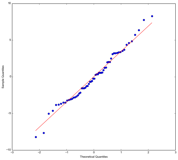

• Save

• Statsmodels 2-Way ANOVA Notebook

Two-way ANOVA in Python using pyvttbl

The third way to perform Python ANOVA is to use the pyvttbl library. Pyvttbl has its own method (also called DataFrame) to create data frames.

from pyvttbl import DataFrame
df = DataFrame()
df.read_tbl(datafile)
df['id'] = xrange(len(df['len']))
print(df.anova('len', sub='id', bfactors=['supp', 'dose']))Code language: Python (python)

The ANOVA tables in Pyvttbl contain much more information than those in statsmodels. Actually, Pyvttbl output contains an effect size measure: the generalized omega squared.

Measure: len

Source	Type III Sum of Squares	df	MS	F	Sig.	η2G	Obs.	SE of x̄	±95% CI	λ	Obs. Power
supp	205.350	1.000	205.350	15.572	0.000	0.224	30.000	0.678	1.329	8.651	0.823
dose	2426.434	2.000	1213.217	92.000	0.000	0.773	20.000	0.831	1.628	68.148	1.000
supp * dose	108.319	2.000	54.159	4.107	0.022	0.132	10.000	1.175	2.302	1.521	0.173
Error	712.106	54.000	13.187
Total	3452.209	59.000

Two-Way ANOVA using Pingouin (Bonus)

Here is a bonus method for performing ANOVA in Python using the Pingouin package. Although pyvttbl is quite good, it is no longer maintained. Here, Pingouin offers a very easy way for ANOVA in Python.

import pandas as pd
import pingouin as pg
data = 'https://vincentarelbundock.github.io/Rdatasets/csv/datasets/ToothGrowth.csv'
df = pd.read_csv(data, index_col=0)
df.head()Code language: Python (python)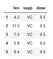

• Save

aov = pg.anova(dv='len', between=['supp', 'dose'], data=df,
             detailed=True)

print(aov)Code language: Python (python)

• Save

• Jupyter Notebook with the Pingouin ANOVA code example