When working with data analysis, one important metric to understand is the SSE in regression, also known as the Sum of Squared Errors. This metric enables us to assess how well our model aligns with the data. It is used not only in simple regression but also in multiple regression and other predictive models.
In this post, we will explain what SSE means, why it matters, and how you can calculate it using R. We will also include an example with code and a short discussion about what SSE represents in regression analysis.
Table of Contents
- What Is SSE in Regression?
- What Does SSE Represent in Regression Analysis?
- How to Calculate SSE in R
- Conclusion
What Is SSE in Regression?
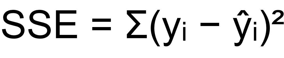
SSE stands for Sum of Squared Errors. It is the sum of the squared differences between the observed values (the actual data) and the predicted values from the regression model. In other words, it indicates the amount of error remaining in the model after fitting the regression line. Here is the formula:
A smaller SSE value indicates that the model’s predictions are close to the actual values. On the other hand, a large SSE may suggest that the model is not accurately capturing the pattern in the data.
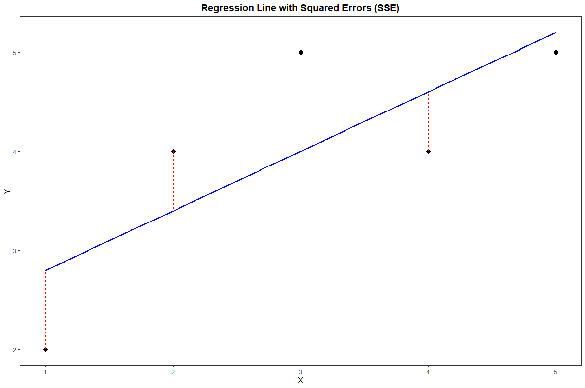
Let’s say you are running a simple linear regression to predict reaction time based on age. Each predicted value will likely differ slightly from the observed value. These differences are called residuals. Squaring each residual and summing them gives you the SSE. This helps quantify how much of the variance is unexplained by your model.
What Does SSE Represent in Regression Analysis?
When asking what does SSE represent in regression analysis, the answer lies in model performance. SSE is a direct measure of model error. It indicates how far the predictions are from the actual values.
SSE is often used in conjunction with other metrics, such as R-squared and Mean Squared Error (MSE). While R-squared gives a proportion of explained variance, SSE gives us the raw amount of unexplained variance. A lower SSE indicates a better fit, assuming we are not overfitting the model by adding unnecessary predictors.
In some cases, researchers also use SSE to compare models. If two models are trained on the same data, the one with the lower SSE may be preferred. However, SSE does not take model complexity into account, so it is not the only metric we should rely on.
How to Calculate SSE in R
Calculating SSE in R is simple. After fitting a linear model, we can extract the residuals and square them to obtain the residuals’ squared values. Here is a quick example using R code:
# Example data
x <- c(1, 2, 3, 4, 5)
y <- c(2, 4, 5, 4, 5)

# Fit a linear model
model <- lm(y ~ x)

# Calculate SSE
sse <- sum(residuals(model)^2)

sseCode language: R (r)
In the code above, we first fit a simple regression model with lm(). We then extract the residuals with residuals(model) and square them using ^2. Finally, we sum them using sum() to get the SSE.
For a more detailed guide, including examples with real datasets and multiple regression, see this post: How to Calculate SSE in R.
Conclusion
To summarize, SSE in regression is a fundamental yet important concept for evaluating model accuracy. It helps us understand how much of the variation in the data is left unexplained by our model. A smaller SSE suggests a better fit, though it should always be interpreted in the context of the full model and other evaluation metrics.
By learning how to calculate and interpret SSE, you take an essential step toward becoming more confident in your regression analyses. Whether we are building models in psychology, behavioral science, or data-driven decision-making, understanding SSE helps us make better and more transparent models. If you found this post helpful, feel free to share it with others and leave a comment below. I would love to hear your thoughts or questions!